Chapter Notes

Quick Overview

Given that this is linear algebra, I will be focusing on linear subspaces, which can be defined as the span, or the amount of space covered by, a finite collection of vectors. These subspaces will lie in $\mathbf{R}^n$, or the space of all n-dimensional vectors(with n coordinates). Linear subspaces will be represented by $\mathsf{V}$. The n-tuples of vectors which define these subspaces will be represented by the following: $\vec{v}_n=\begin{bmatrix} \vec{v}_1 \\ \vdots \\ \vec{v}_n \end{bmatrix}$

Chapter 1: Vectors

Vector Overview

Vectors can represent a very wide variety of things from physical direction and magnitude to collections of numerical data. In other words, vectors are typically thought of as representing a particular direction, but they don’t always have to denote movement or incremental distance along coordinate axis.

This is especially true for problems in data science where there are large collections of numerical data that would be easier to work with if put into vector form. For example, say we wanted to keep track of the precipitation amount each day at Stanford over the course of a year. We could organize this data into a 365-vector: $\mathbf{P}=\begin{bmatrix} P_1 \\ P_2 \\ \vdots \\ P_{365} \end{bmatrix}$ We have a general idea for defining vectors but provided below is a more concrete definition which clarifies what I meant by a “365-vector”.

Definition 1.1.2: For a whole number n, an n-vector is a list of n real numbers. We denote by $\mathbf{R}^n$ the collection of all possible n-vectors.

Additionally, we can introduce the idea of a scalar, which can be understood by the following definition provided below.

Definition 1.1.4: To distinguish ordinary real numbers from vectors, the word scalar refers to a real number.

So we know what vectors and scalars are but what can we do with them? How can we manipulate and combine them?

Definition 1.3.1: The sum $\vec{v}$ + $\vec{w}$ of two vectors is defined precisely when $\vec{v}$ and $\vec{w}$ are n-vectors for the same n. In that case, we define their sum by the rule:$\begin{bmatrix} \vec{v}_1 \\ \vdots \\ \vec{v}_n \end{bmatrix}$ + $\begin{bmatrix} \vec{w}_1 \\ \vdots \\ \vec{w}_n \end{bmatrix}$ = $\begin{bmatrix} \vec{v}_1 + \vec{w}_1 \\ \vdots \\ \vec{v}_n + \vec{w}_n \end{bmatrix}$

Definition 1.3.2 We multiply a scalar c against an n-vector v = $\vec{v}_n=\begin{bmatrix} \vec{v}_1 \\ \vdots \\ \vec{v}_n \end{bmatrix}$ by the rule $c\vec{v}_n=\begin{bmatrix} c\vec{v}_1 \\ \vdots \\ c\vec{v}_n \end{bmatrix}$.

Definition 1.3.4 A linear combination of two n-vectors $\vec{v}$, w is an n-vector $a\vec{v}$ + $b\vec{w}$ for scalars a, b. More generally, a linear combination of k such n-vectors $ v_1, v_2,…,v_k$ is $a_1v_1 + a_2v_2 + ··· + a _kv_k $ for scalars $a_1, a_2, . . . , a_k.$

Linear combinations, or vector addition can be interpreted through a parallelogram rule. This is a nice geometric interpretation of vector addition which showcases the commutative property of vector addition. Below I have provided an image which nicely visualizes this parallelogram rule:

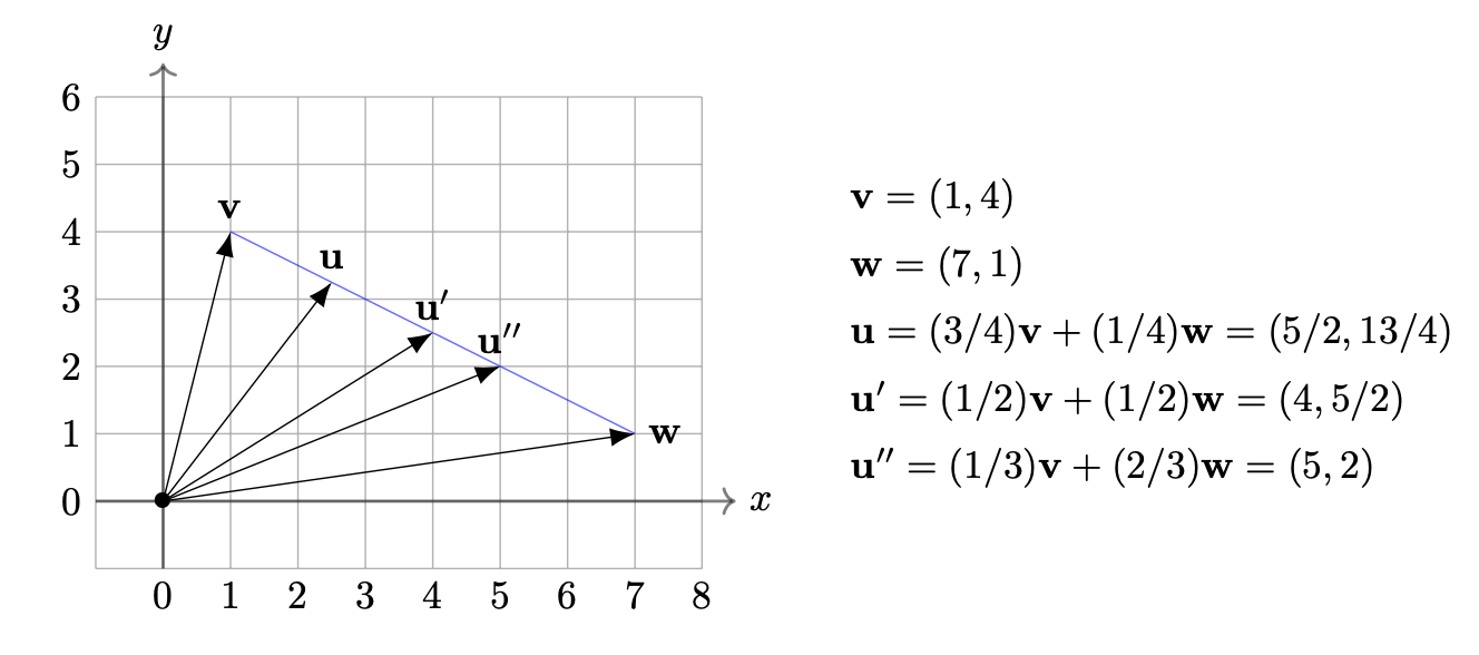
Convex Linear Combinations: These Linear combinations involve two n-vectors $\vec{v}$ and $\vec{w}$. This linear combination of these vectors can be written in the form $(1 − t)\vec{v} + t\vec{w} = \vec{v} + t(\vec{w} − \vec{v})$ with $0 ≤ t ≤ 1$. This adds to $\vec{v}$ a portion(given by t) of the displacement $\vec{w}$ − $\vec{v}$ from $\vec{v}$ to w. For $\mathbf{R}^2$ and $\mathbf{R}^3$ it can be interpreted as being a point on the line segment between the tips of $\vec{v}$ and $\vec{w}$; e.g., it is $\vec{v}$ when t = 0, it is the midpoint when t = 1/2, and it is $\vec{w}$ when t = 1.

Here’s an image to help visualize how t changes the influence each vector has on the linear combination:

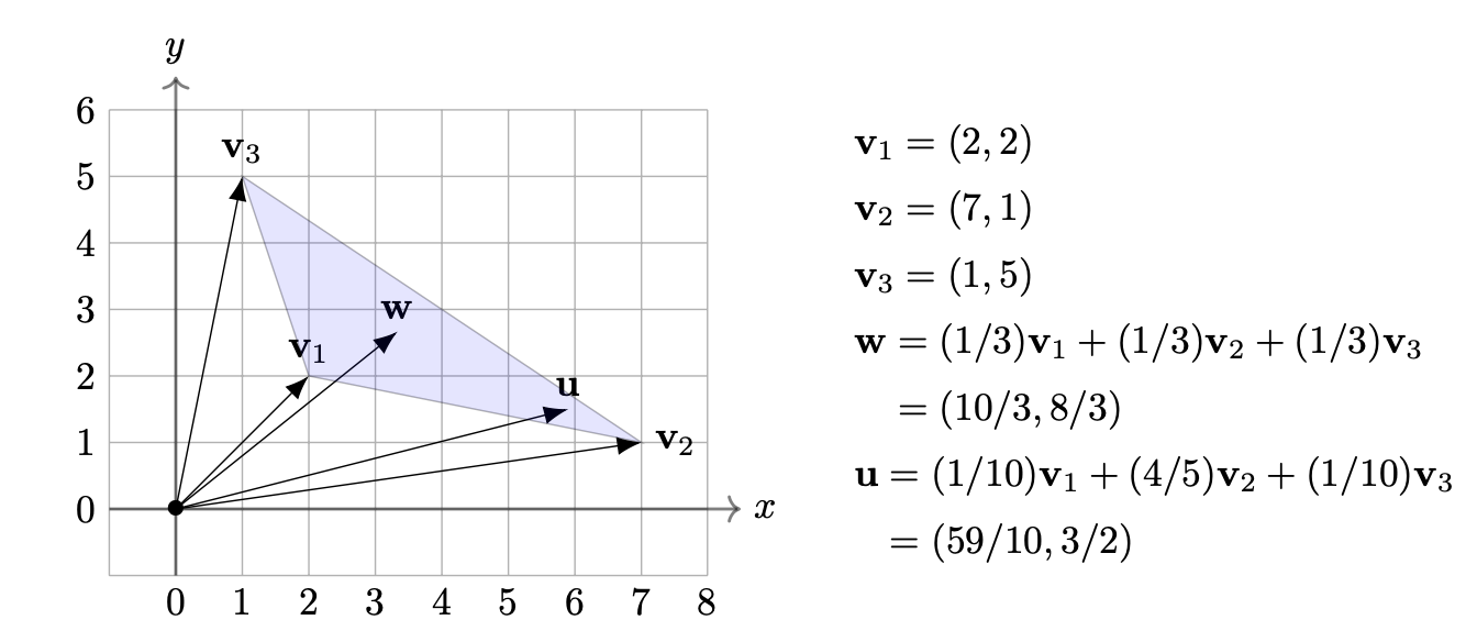
For any n-vectors $v_1 , . . . , v_k$ , a convex combination of them means a linear combination $t_1v_1 + ··· + t_kv_k$ for which all $t_j≥0$ and the sum of the coefficients is equal to 1; that is, $t_1 + ··· + t_k =1$. When the k coefficients are all equal, which is to say every $t_j$ is equal to 1/k, this is the centroid of the k vectors. It’s essentially just the average of the k vectors. Working in $\mathbf{R}^2$, a convex combination where not all coefficients are equal is a point inside the polygon with vertices given by the $v_j$’s, with its distance to each $v_j$ weighted by the corresponding coefficient. If all coefficients are equal, it is the “center of mass” of the polygon defined by the vectors.

This is better interpreted by images, so take a look at this awesome screenshot from my textbook :)

Vector Algebra: As I stated earlier vector addition follows the commutative law. That is $\vec{v} + \vec{w} = \vec{w} + \vec{v}$. This is, at least in my eyes, trivial so I do not feel the need to justify this law. This applies to all Rn(Latex) and applies to the addition of more than just 2 vectors(associativity).

Definition 1.6.1 The length or magnitude of an n-vector $\vec{v}$ = $\vec{v}_n=\begin{bmatrix} \vec{v}_1 \\ \vdots \\ \vec{v}_n \end{bmatrix}$, denoted ∥$\vec{v}$∥, is the number $∥ v ∥ = \sqrt{v_1^2 + v_2^2 + · · · + v_n^2} ≥ 0$. Note that the length is a scalar, and ∥$-\vec{v}$∥ = ∥$\vec{v}$∥ (in accordance with the visualization of $-\vec{v}$ as “a copy of $\vec{v}$ pointing in the opposite direction”) because signs disappear when squaring each $-\vec{v}_j$ . If c is any scalar then ∥$c\vec{v}$∥ = |c|∥$\vec{v}$∥ (i.e., if we multiply a vector by c then the length scales by the factor |c|). For example, (−5)$\vec{v}$ has length 5∥$\vec{v}$∥. (In other references, you may see ∥$\vec{v}$∥ called the “norm” of $\vec{v}$.)

Definition 1.6.4: The distance between two n-vectors $\vec{x}$, $\vec{y}$ is defined to be $∥\vec{x} − \vec{y}∥$. (This will soon be visualized as the familiar notion of distance between tips of arrows for n = 2, 3. In general, it also equals $∥\vec{y} − \vec{x}∥$ since $y − x = −(x − y)$ and any vector has the same length as its negative, so the order of subtraction doesn’t matter.

Definition 1.7.1: The zero vector in $\mathbf{R}^2$ is $0 = \begin{bmatrix} 0 \\ \vdots \\ 0 \end{bmatrix}$, and a unit vector is a vector pointing in the same direction as $\vec{v}$ with length one, found using the following: $\vec{u}=\frac{\vec{v}}{∥\vec{v}∥}$. Always ∥$\vec{v}$∥ ≥ 0, and $∥\vec{v}∥ = 0$ precisely when $\vec{v}$ = 0.

Include here some worked examples

Chapter 2

From here on we will see my lack of time become…apparent in terms of the quantity of notes produced. However, I will try to make up for that with quality :).

Vector Geometry and Correlation Coefficients

In this section I will cover how the dot product can be used to develop a geometric understanding for $\mathbf{R}^n$. I will start by discussing the dot product in $\mathbf{R}^2$ & $\mathbf{R}^3$, then I will generalize to n > 3.

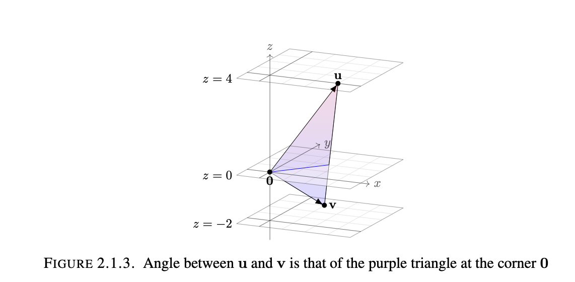
Definition 2.1.1: In $\mathbf{R}^2$ the angle between two vectors: $a=(a_1, a_2)$ & $b=(b_1, b_2)$ can be related by $\cos(\theta)=\frac{a_1b_1+a_2b_2}{||a||||b||}$

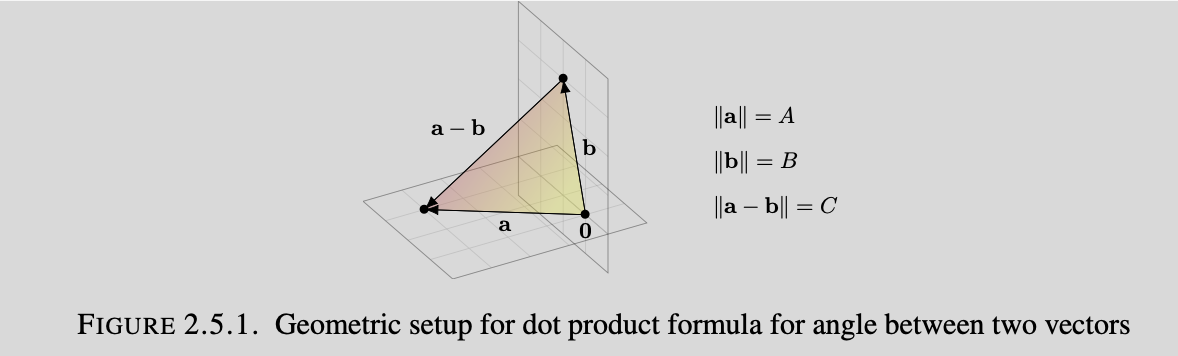
This may seem strange, but it is actually just a re-arranged form of the law of cosines. Imagine a triangle formed by the vectors $a$, $b$, and $(a-b)$. We will refer to $a$ as side $A$, $b$ as side $B$, and $(a-b)$ as side $C$. The law of cosines says $C^2=A^2+B^2-2AB\cos(\theta)$. We can rearrange this to $\cos(\theta)=\frac{A^2+B^2-C^2}{2AB}$. Putting the numerator and denominator in terms of the vector form gives us $\cos(\theta)=\frac{(a_1^2+a_2^2)+(b_1^2+b_2^2)-((a_1-b_1)^2+(a_2-b_2)^2)}{2||a||||b||}$ This simplifies out to the result above. This method of finding the angle between two vectors can be generalized to n dimensions by the dot product.

Definition 2.1.6: Consider n-vectors $\vec{x}=\begin{bmatrix} \vec{x}_1 \\ \vdots \\ \vec{x}_n \end{bmatrix}$ & $\vec{y}=\begin{bmatrix} \vec{y}_1 \\ \vdots \\ \vec{y}_n \end{bmatrix}$.

(i) The dot product of x and y is defined to be the scalar: $x \cdot y=x_1y_1+x_2y_2+…+x_ny_n=\sum_{i=1}^{n} x_iy_i$ (The dot product is only defined if the two vectors are n-vectors for the same value of n.)

(ii) The angle $\theta$ between two nonzero n-vectors x, y is defined by the formula: $\cos(\theta)=\frac{x \cdot y}{||x||||y||}$ With 0° ≤ $\theta$ ≤ 180°

(iii) When $x \cdot y=0$, x and y are perpendicular/orthogonal

Here’s an image to help visualize:

Some properties of the dot product naturally follow:

$v \cdot v= v_1^2+v_2^2+…+v_n^2=||v||^2\geq 0$ with equality exactly at when v=0

Cauchy-Schwarz Inequality: $|x \cdot y|\leq||x||||y||$

This results from looking at the other helpful formulation of the dot product: $x \cdot y=\cos(\theta)||x||||y||$. As we can see, if we take the absolute value, the cosine in the formula will only ever give values $0\leq\cos(\theta)\leq1$ therefore the dot product will always be capped by the magnitude of the first vector multiplied by the magnitude of the second(when cosine is at 0).

Theorem 2.2.1: For any n-vectors v, w, $w_1$, $w_2$, the following hold:

(i) $v \cdot w=w \cdot v$

(ii) $v \cdot v=||v||^2$(already referenced above)

(iii) $v \cdot (cw) = c(v \cdot w)$ for any scalar c, and $v \cdot (w_1+w_2)=v \cdot w_1 + v \cdot w_2$

(iii’) Combining both rules in (iii), for any scalars c_1, c_2 we have $v \cdot (c_1w_1 + c_2w_2)=c_1(v \cdot w_1) + c_2(v \cdot w_2)$

These can be generalized to larger n: $v \cdot w=\sum_{i=1}^{n}v_iw_i=w \cdot v=\sum_{i=1}^{n}w_iv_i$

Here’s an example of using the dot product with larger n:

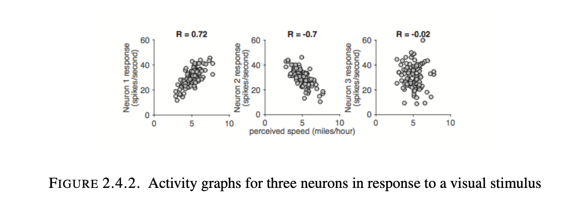
Correlation Coefficients: Given data points $(x_1,y_1),(x_2,y_2),…(x_n,y_n)$, it is often useful to find a line of best fit for the data. But to determine whether it is even worth finding a best fit line, it is useful to see if there is a linear relationship between the $x_i$’s and the $y_i$’s. The correlation coefficient, r, measures such linear relation.

Definition 2.2.3: Consider a set of n data points $(x_1,y_1),(x_2,y_2),…(x_n,y_n)$. $X=\begin{bmatrix} \vec{x}_1 \\ \vdots \\ \vec{x}_n \end{bmatrix}$, $Y=\begin{bmatrix} \vec{y}_1 \\ \vdots \\ \vec{y}_n \end{bmatrix}$ The correlation coefficient between the $x_i$’s and the $y_i$’s is the cosine of the angle between x and y: or $r=\frac{X \cdot Y}{||X||||Y||}$

Some examples of correlation coefficients:

Add examples and a few other things

Chapter 3

Planes

In this section I will discuss planes in $\mathbf{R}^3$. In particular, I will discuss the different descriptions of planes, the transition between different forms of writing an equation for a plane, determine if points lie on the same side or different sides of a plane, and interpreting the parametric form in terms of displacement vectors from a point on the plane.

Definition 3.1.1: The collection of points (x, y, z) in $\mathbf{R}^3$ satisfying an equation of the form $ax+by+cz=d$ is known as a plane. At least one of the constants a, b, or c must be non-zero.

Equational Form: $\large ax+by+cz=d$

-This form describes the set of all x, y, and z that lie on the plane. It will also be useful in determining whether 2 or more points are on the same side of a plane.

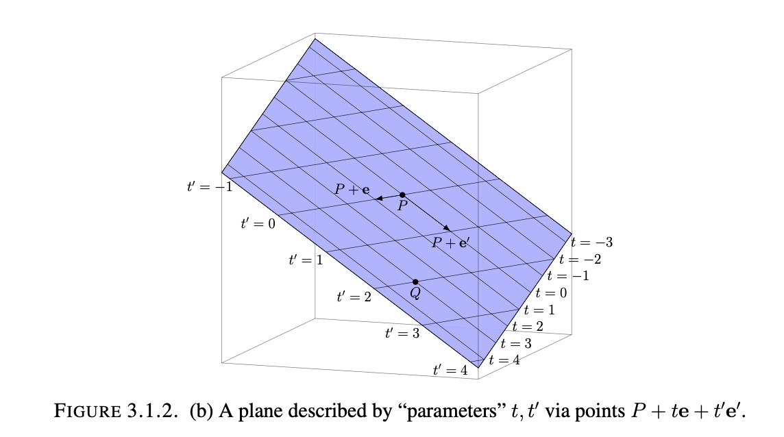
Parametric Form: $\large \begin{bmatrix} p_1 \\ p_2 \\ p_3 \end{bmatrix} + t\begin{bmatrix} v_1 \\ v_2 \\ v_3 \end{bmatrix} + t’\begin{bmatrix} w_1 \\ w_2 \\ w_3 \end{bmatrix}$

-This form describes the set of all points on the plane as the linear combination of some initial point, P, lying on the plane, with two independently-scaled vectors v and w which describe two directions on the plane. Note that these vectors do not have to be perpendicular, since the set of all linearly independent vectors span the entire plane that they lie on.

Point and Normal Vector Form: $\large P=\begin{bmatrix} p_1 \\ p_2 \\ p_3 \end{bmatrix}$ and $\large n=\begin{bmatrix} n_1 \\ n_2 \\ n_3 \end{bmatrix}$

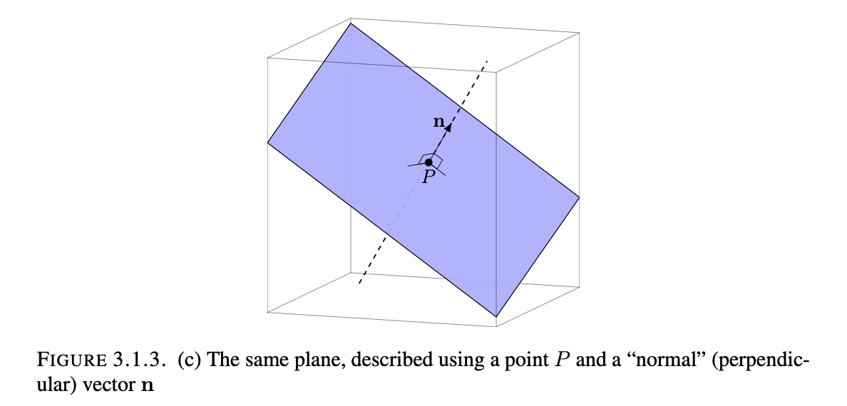
-This isn’t a complete form on it’s own, rather it is actually the basis for the equational form of a plane, but it is helpful to visualize the plane in terms of the normal vector and the point which define the set of all other points on the plane. In-fact for the equational form the coefficients a, b, and c are all determined by the normal vector n where $(n_1, n_2, n_3)$ represent a, b, and c respectively. Finally, d is found by plugging in point P for x, y, and z and evaluating the result. Note that the vectors used must not be scalar multiples of each other.

Other Ways the Information to Form a Plane Might be Given: Sometimes the information necessary to form a plane might be given by three points P, Q, R. Two find an equation for a plane with this information, all that is necessary is to pick some initial point, say P(will also serve as initial point for parametric form), then find the direction vectors from P to Q and P to R. After, you can either take the parametric path by organizing $\vec{PQ}$ and $\vec{PR}$ and using the initial point P to reach the form $P + t\vec{PQ} + t’\vec{PR}$, or you can take the equational/normal form by finding the normal vector $n$. $n$ can be found by creating an arbitrary vector $\vec{n}=\begin{bmatrix} n_1 \\ n_2 \\ n_3 \end{bmatrix}$ and setting up a system of equations that modeled by the dot product of it with each vector(making sure to set the dot product to zero. By doing so, values of $n_1, n_2, and n_3$ can be found which, when dotted with each vector is zero, therefore proving that $\vec{n}$ is orthogonal to the plane. Then using $n_1, n_2, and n_3$ for a, b, and c, we can find the equational form after plugging in the initial point P for x, y, and z.

Additionally, you may be provided with the normal vector of the plane, and you may be asked to find the parametric form of the plane. To do this, write the equational form of the plane then restrict either x or y or z to be zero, then set one of the others to be 1, then evaluate what the last variable must be to lie on the plane. Repeat to obtain a third point then create the directional vectors necessary to write the parametric form of the equation. We should make sure that the coefficient of that third variable solved at the end is not 0.

Describing a Line in Parametric Form: A line in parametric form can be expressed through a vector, $p$, which specifies a point the line originates from, and
a scaled vector $tv$. We can visualize this scaled vector as the actual line, where each segment is made up of a different scalar t, and the entire line is made up by the set of all scalars t.

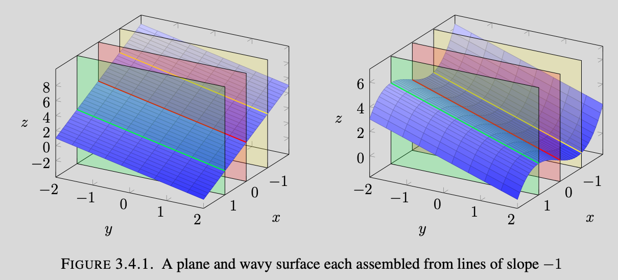
This form can help us understand the equational form of planes. With a manipulation of variables we can express the plane as z in terms of x and y, then we can fix x or y. Visualizing the set of same-sloped lines created when fixing one of these variables and evaluating the expression at various values of the fixed variable will result in a plane becoming clear. However, there are multiple non-planar surfaces that can create such a set of lines when performing this process, therefore we must make a distinction. The lines created by these planes will have the same slope, and the rate by which their height varies at a linear rate.

Add examples and images

Chapter 4

Span, Subspaces, and Dimension

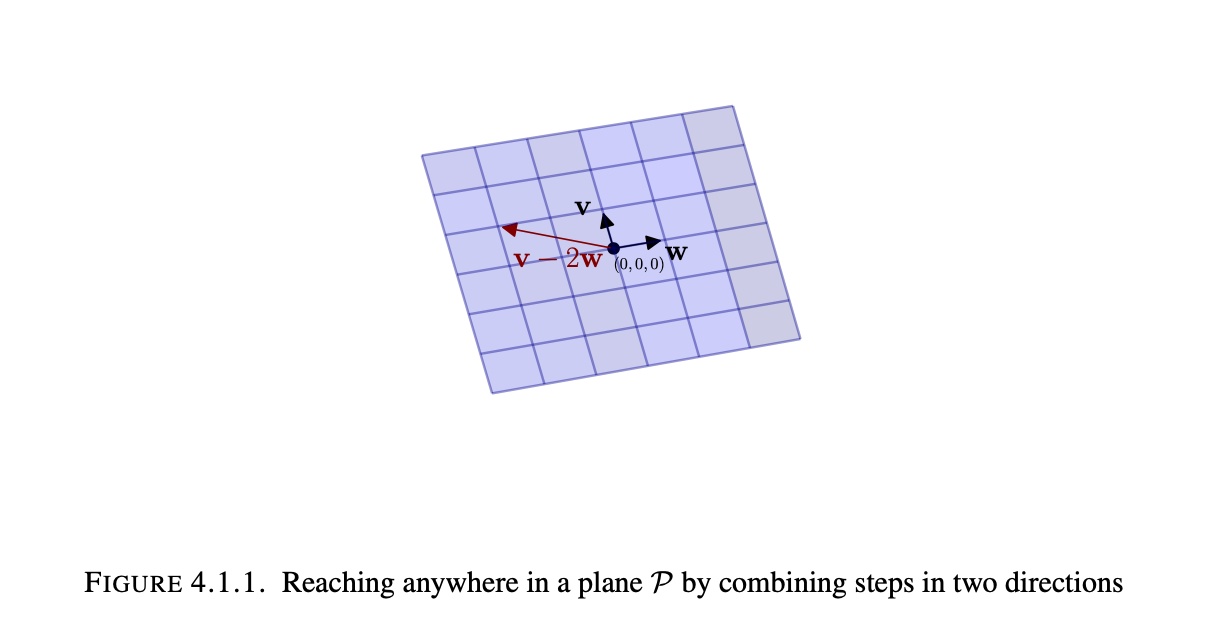
When given a set of n-vectors in Rn, oftentimes it is useful to look at the space that could be covered by the set of all linear combinations of those vectors. This space is defined as the span of those n-vectors. For example given a plane in R3 passing through 0=(0, 0, 0). We want to mathematically express the idea that the plane is flat with 2 degrees of freedom. By choosing two vectors v & w that do not lie on a common line through 0 we can map out every point in the plane as a combination of scalar multiples of the vectors v and w. In other words, plane: $P = {all vectors of the form av + bw, for scalars a, b}$. If any n n-vectors happen to be scalar multiples of each other, they are defined as being linearly dependent and thus, they lay on the same line with span defined by a scalar multiplied by the direction vector of the line.

Definition 4.1.3: The span of vectors $v_1, …,v_k$ in Rn is the collection of all vectors in Rn that one can obtain from $v1, …, vk$ by repeatedly using addition and scalar multiplication. In symbols:$span(v_1, …,v_k)=${alln-vectors x of the form $c_1v_1+…+c_kv_k$} where $c_1, …,c_k$ are arbitrary scalars.

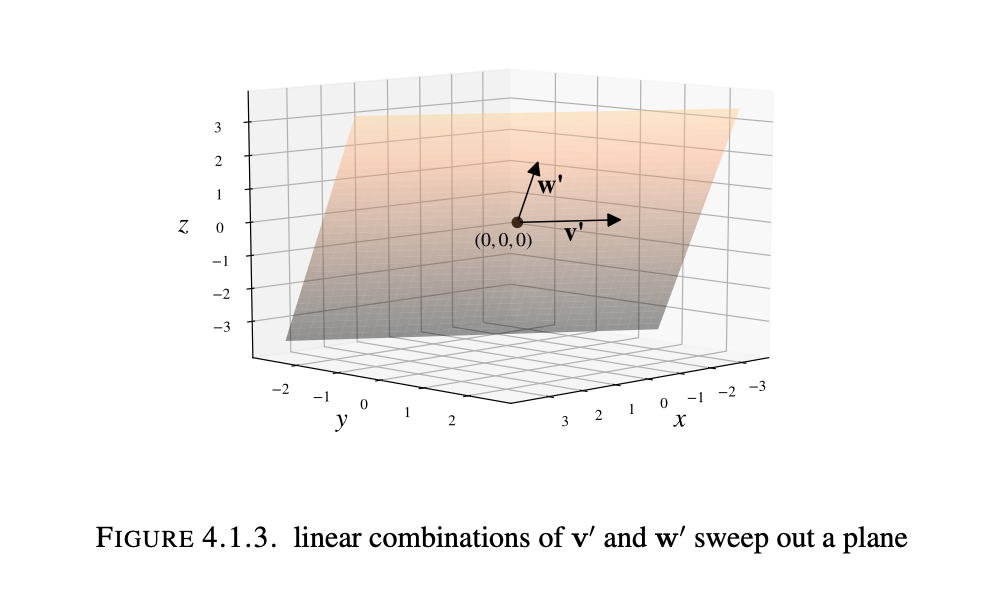
In R3, for k=2 and nonzero $v_1$, $v_2$ not multiples of each other, this recovers the parametric form of a plane through P = 0. In general, the span of a collection of finitely many n-vectors is the collection of all the n-vectors one can reach from those given n-vectors by forming linear combinations in every possible way.

The span of two nonzero n-vectors that are not scalar multiples of each other should be visualized as a plane through 0 in Rn(assuming n is not 1). With larger Rn and larger sets of vectors we will discuss visualizing/understanding their span.

The set of vectors in Rn perpendicular to any fixed nonzero vector in Rn is a span of n-1 nonzero n-vectors. As we know in R3 the set of vectors perpendicular to a 3-vector is the span of 2 3-vectors(a plane).

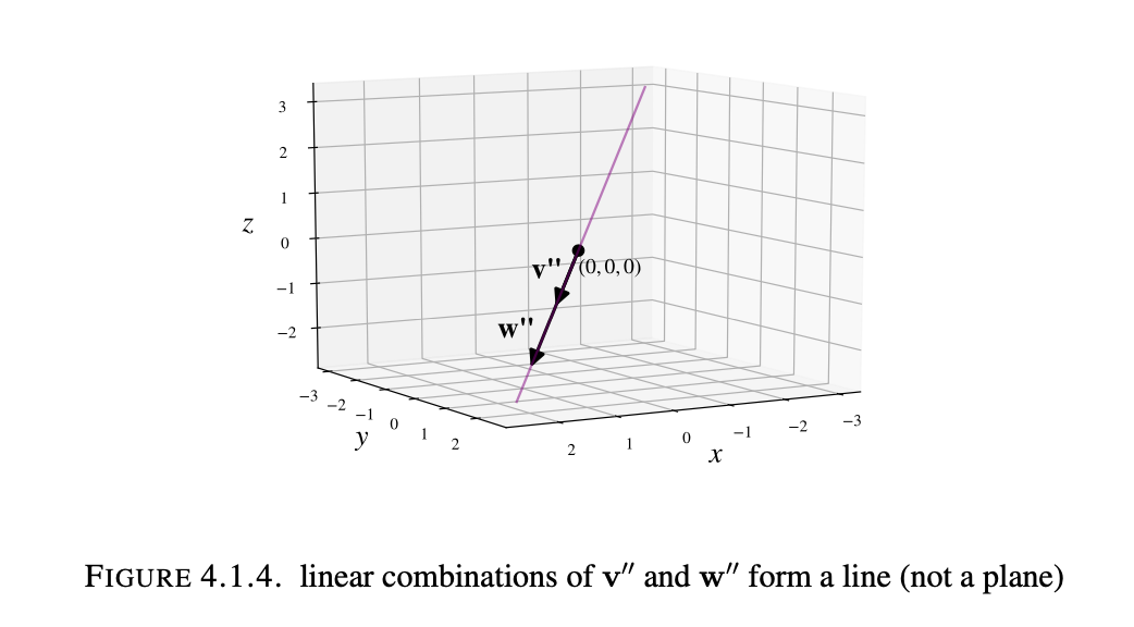
A line in R2 or R3 passing through 0 and a plane in R3 passing through 0 each arise a span of one or two vectors. But lines and planes not passing through 0 are not a span of any collection of vectors since the span of any collection of n-vectors always contains 0, by setting all coefficients $c_1, …, c_k$ in Definition 4.1.3 to be 0.

If V is the span of some finite collection of vectors in Rn then there are generally many different sets of vectors that have the same span.

Add in example discussing the 4-vectors that amre perpendicular to another vector

Definition 4.1.7: A linear subspace of Rn is a subset of Rn that is the span of a finite collection of vectors in Rn. If V is a linear subspace of Rn, a spanning set for V is a collection of n-vectors v1, …, vk whose span equals V.

Affine Subspaces: Sometimes a line or plane will not pass through the origin, and we will want to discuss the space which the composite vectors describe. We define such a space as an affine subspace although the concept is surprisingly less practical than linear subspaces.

Proposition 4.1.11: If V is a linear subspace in Rn, then for any vectors $x_1, …, x_m$ lying in $V$ and scalars $a_1,…,a_m$ the linear combination $a_1x_1+…+a_mx_m$ also lies in V. What follows is that in order to check if a set is a linear subspace, we must make sure it satisfies the conditions of a linear subspace: all cV and V+W make up the set.

To determine if some equation represents a linear subspace what I need to do is find some points/vectors (x,y,z) that satisfy the conditions of the equation then verify whether they: contain the zero vector; can be scaled and still satisfy the equation, and can be added and still satisfy the equation

Include example 4.1.13 Namely explain why they first rewrite the perpendicularity equations in terms of three variables then explain how that relates to the span of vectors that are perpendicular to the two vectors. Answer: the perpendicular vector we solved for represents the linear combination of three scaled vectors with scalars x_2, x_4, and x_5 which makle up all the normal vectors to the other two vectors.

Example Problem: Consider the set W of all vectors in c that are perpendicular to both $\begin{bmatrix} 1 \\ 1 \\ 0 \\ -1 \\ 2 \end{bmatrix}$ and $\begin{bmatrix} 0 \\ 2 \\ 3 \\ 1 \\ -1 \end{bmatrix}$.

We will now find three explicit 5-vectors $v_1, v_2, v_3$ so that W = span($v_1, v_2, v_3$), and in particular W is a linear subspace of $\mathbf{R}^5$. (This phenomenon is not specific to W; it works for perpendicularity against any finite collection of vectors in any $\mathbf{R}^n$. This can be explained by relating the algebra and geometry of linear algebra: showing that the solution to any such system of conditions is a span of a finite set of vectors.) Now we write out the two perpendicularity requirements in terms of dot products. Namely, a vector $\begin{bmatrix} x_1 \\ x_2 \\ x_3 \\ x_4 \\ x_5 \end{bmatrix}$ in $\mathbf{R}^5$ lies in W precisely when it satisfies the two “perpendicularity equations” $$x_1 + x_2 - x_4 + 2x_5 = 0, 2x_2 + 3x_3 + x_4 - x_5 = 0$$. We can rewrite these two equations as expressing two of the variables in terms of the others (with no further constraints in these other variables), say $x_1, x_3$ in terms of $x_2, x_4, x_5$: the pair of equations equivalently says $$x_1=-x_2+x_4-2x_5, x_3=-(2/3)x_2-(1/3)x_4+(1/3)x_5$$. Since there are no restrictions at all on $x_2, x_4, x_5$, W is the collection of vectors of the form $\begin{bmatrix} -x_2 + x_4 - 2x_5 \\ x_2 \\ -(2/3)x_2 - (1/3)x_4 + (1/3)x_5 \\ x_4 \\ x_5 \end{bmatrix}$ for arbitrary scalars $x_2, x_4, x_5$. This vector can be expressed in the form of a linear combination by separating out the parts involving each $x_2, x_4, x_5$ separately: $\begin{bmatrix} -x_2 \\ x_2 \\ -(2/3)x_2 \\ 0 \\ 0 \end{bmatrix}$ + $\begin{bmatrix} x_4 \\ 0 \\ -(1/3)x_4 \\ x_4 \\ 0 \end{bmatrix}$ + $\begin{bmatrix} -2x_5 \\ 0 \\ (1/3)x_5 \\ 0 \\ x_5 \end{bmatrix}$ = $x_2\begin{bmatrix} -1 \\ 1 \\ -(2/3) \\ 0 \\ 0 \end{bmatrix}$ + $x_4\begin{bmatrix} 1 \\ 0 \\ -(1/3) \\ 1 \\ 0 \end{bmatrix}$ + $x_5\begin{bmatrix} -2 \\ 0 \\ (1/3) \\ 0 \\ 1 \end{bmatrix}$.

In other words, W is the span of vectors $v_1=\begin{bmatrix} -1 \\ 1 \\ -(2/3) \\ 0 \\ 0 \end{bmatrix}$, $v_2=\begin{bmatrix} 1 \\ 0 \\ -(1/3) \\ 1 \\ 0 \end{bmatrix}$, $v_3=\begin{bmatrix} -2 \\ 0 \\ (1/3) \\ 0 \\ 1 \end{bmatrix}$.

Now we will move on to discussing dimension. A good way of understanding the dimension of something is to consider the collection P4 of all polynomials of degree at most 4. Such a polynomial has the form $ax^4+bx^3+cx^2+dx+e$ where all constants can be any real numbers. This description involves 5 independent choices(a,b,c,d,e). Essentially this means P4 is 5 dimensional since it can be defined by 5 numbers. Informally, the “dimension” of an object X tells us how many different numbers are needed to locate a point in X.

Now with this general idea we can better articulate this to be less ambiguous and more useful. We will do this by focusing on the case of a linear subspace V of Rn, where vector algebra will provide a way to make that informal idea precise. The “dimension” of V will be, intuitively, the number of independent directions in V. In other words, it will tell us how many numbers we need in order to specify a vector v in V.

Definition 4.2.4: Let V be a nonzero linear subspace of some Rn. The dimension of V, denoted as dim(v), is defined to be the smallest number of vectors needed to span V. We define dim({0})=0.

Theorem 4.2.5: For $k\geq 2$, consider a collection $v_1,…,v_k$ of vectors spanning a linear subspace V in Rn. We have dim(V)=k precisely when there is no redundancy, or when each $v_i$ is not a linear combination of the others(removing one destroys the spanning property). Equivalently, dim(V)<k precisely when “there is redundancy”: some $v_i$ is a linear combination of the others, or in other words removing it will not affect the span.

Theorem 4.2.8: If V and W are linear subspaces of Rn with W contained in V(every vector in W also belongs to V) then dim(W)$\leq$dim(V)

Dimension Criterion: Span of two vectors: a subspace span(u,v) has dimension 2 if u and v are not collinear. Span of three vectors: a subspace V = span(u,v,w) has dimension three except when: -all vectors are collinear. Then dim(V)=1. -two of the three vectors are collinear. Then dim(V)=2. -None of the vectors are collinear, but one of them is a linear combination of the two others. Then dim(V)=2.

Chapter 5

Basis and orthogonality

Definition 5.1.1: A basis of a subspace V of Rn is a spanning set of V that has exactly k=dim(V) n-vectors. i.e. a spanning set with as few vectors as possible in it.

Since a linear subspace has many spanning sets, it has many bases. For example, if {u,v,w} is a basis of V, then so is {-u,2v,v+W}, BUT NOT {2u,-v+w} since it has only 2 n-vectors defining 3-space–NOR IS {-u,2v,u-4v} since its vectors do not include w. Also, any set of 4 3-vectors in this example would not be considered a basis because it is not the least number of vectors necessary to define the linear subspace.

To see if any given set of k n-vectors has $dim(v) <$ span$(v_1,v_2, …, v_k)$ we can simply pick one $v_i$ and pick arbitrary scalars $c_1, …,c_k$ not including $c_i$ then we can set $v_i$ equal to the linear combination of the other scaled vectors to set up a system of equations. With this system of equations we can find the potential linear combinations that result in vector $v_i$ proving that $dim(v) <$ span$(v_1,v_2, …, v_k)$. If the set of k n-vectors is a basis for V, then there will be no such set of scalars which result in a linear combination that equals $v_i$. Later on we will find a way to remove redundancy for a spanning set for a linear subspace V of Rn, but for now this is all we have lol. The next type of spanning set for any linear subspace V is always guaranteed to be a basis of V.

Definition 5.2.1: A collection of vectors $v_1,v_2, …, v_k$ in Rn is called orthogonal if $v_i\cdot{v_j}=0$ whenever i is not equal to j. I.e. all the vectors are perpendicular to one another.

Theorem 5.2.2: If $v_1,v_2, …, v_k$ is an orthogonal collection of nonzero vectors in Rn then it is a basis for span($v_1,v_2, …, v_k$). In particular, span($v_1,v_2, …, v_k$) Then has dimension k, and we call $v_1,v_2, …, v_k$ an orthogonal basis for its span. (A single nonzero vector is always an orthogonal basis for its span)

The span of a collection of k vectors in Rn has dimension of at most k. By theorem 5.2.2, orthogonality is a useful way to guarantee that k given nonzero n-vectors have a k-dimensional span.

Include example 5.2.4

Theorem 5.2.5: Every nonzero linear subspace of Rn has an orthogonal basis. There is an especially convenient type of orthogonal basis for every type of orthogonal basis for a nonzero linear subspace of Rn included in definition 5.2.6

Definition 5.2.6: A collection of vectors $v_1,v_2, …, v_k$ in Rn is called orthonormal if they are orthogonal to each other and in addition they are all unit vectors; that is $v_i\cdot{v_i}=1$ for all i (ensuring $||v_i||=\sqrt{v_i\cdot{v_i}}=\sqrt{1}=1$ for all i).

Any orthonormal collection of vectors is a basis of its span, by theorem 5.2.2.

It is worth noting that it is not always useful to try and solve a system of equations to find the dimension of some set of vectors spanning V to see if they are a basis. In those cases where there are many unknowns and many equations, it may be more useful to simply check if the vectors are orthogonal.

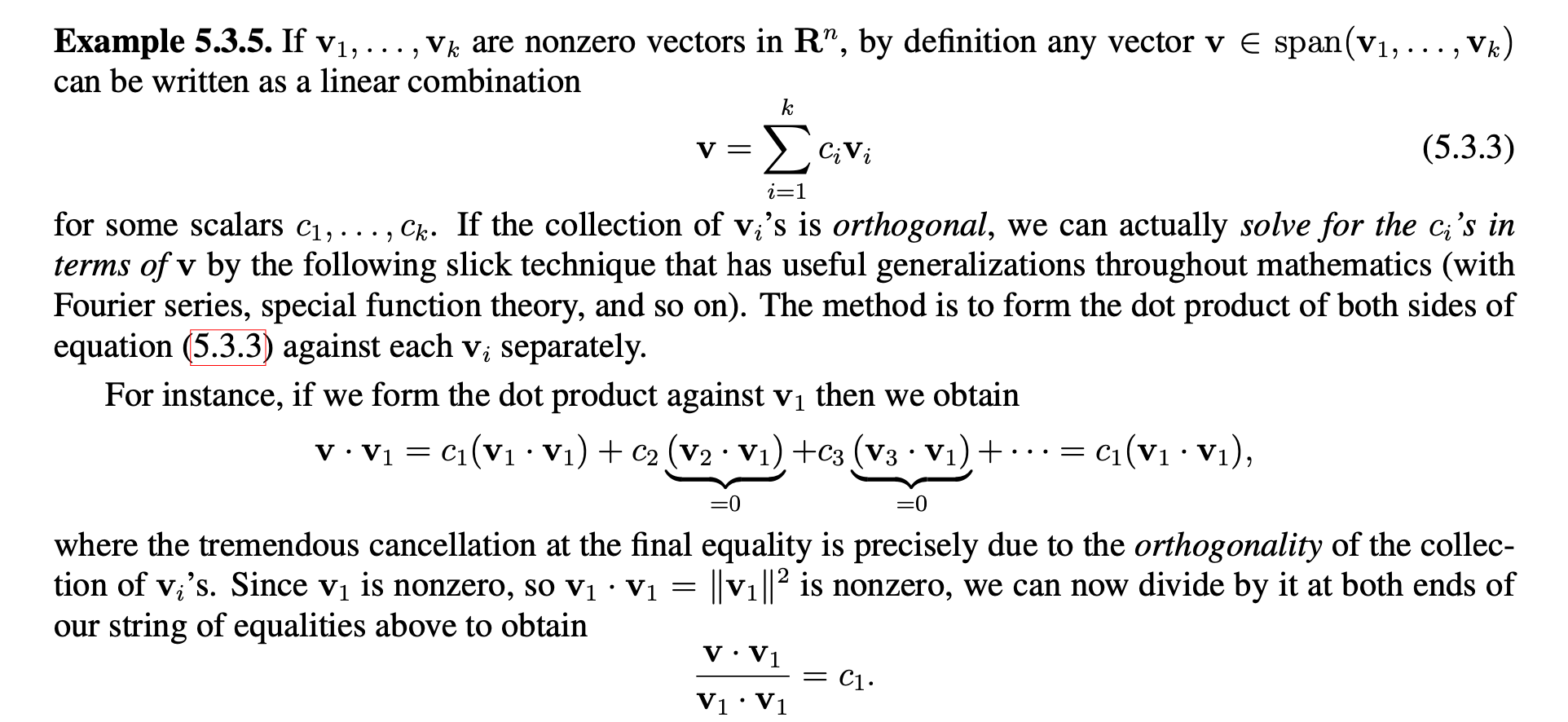
Theorem 5.3.6(Fourier Formula): For any orthogonal collection of nonzero vectors $v_1,v_2, …, v_k$ in Rn and vector v in their span, $$v=\sum_{i=1}^k(\frac{v\cdot{v_i}}{v_i\cdot{v_i}}v_i$$ In particular, if the $v_i$’s are all unit vectors (so $v_i\cdot{v_i}=1$ for all i) then $v=\sum_{i=1}^k(v\cdot{v_i}v_i$.

This is basically just a nice formula for finding what linear combination of basis vectors gives another specific vector within the span of the basis vectors.

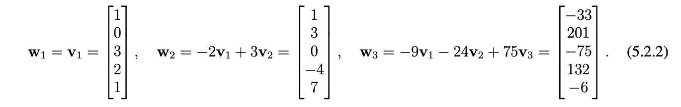
Example 5.3.8: Consider the explicit orthogonal basis ${w_1, w_2, w_3}$ for the linear subspace $V=span(v_1,v_2,v_3)$ in $\mathbf{R}^5$ with explicit $v_i$’s provided below.

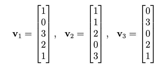
(Note that in this case the orthogonal basis of $w_i$’s is given, we will learn how to solve later

Applying the Fourier formula for the orthogonal basis ${w_1,w_2,w_3}$ of V, for each $v \in V$ we have $$v=\sum_{i=1}^3(\frac{(v\cdot{w_i})}{(w_i\cdot{w_i})})w_i=(\frac{(v\cdot{w_1})}{15})w_1+\frac{v\cdot{w_2}}{75}w_2+\frac{v\cdot{w_3}{64575}w_3$$ since the denominators in the final expression are just the dot product evaluations $w_1 \cdot{w_1}=15$, $w_2 \cdot{w_2}=75$, $w_3 \cdot{w_3}=64575$.

Consider the vector $v=2v_1-v_2+v_3=\begin{bmatrix} 2 \\ 0 \\ 6 \\ 4 \\ 2 \end{bmatrix} - \begin{bmatrix} 1 \\ 1 \\ 2 \\ 0 \\ 3 \end{bmatrix} + \begin{bmatrix} 0 \\ 3 \\ 0 \\ 2 \\ 1 \end{bmatrix} = \begin{bmatrix} 1 \\ 2 \\ 4 \\ 6 \\ 0 \end{bmatrix}$ in $V$. Since ${w_1,w_2,w_3}$ is a basis of V, we know that there is some expression of the form $v=c_1w_1+c_2w_2+c_3w_3$ for unknown scalars $c_1,c_2,c_3$. These scalars can be solved for using a brute-force system of equations: $$\begin{bmatrix} 1 \\ 2 \\ 4 \\ 6 \\ 0 \end{bmatrix}=v=c_1w_1+c_2w_2+c_3w_3=c_1\begin{bmatrix} 1 \\ 0 \\ 3 \\ 2 \\ 1 \end{bmatrix} + c_2\begin{bmatrix} 1 \\ 3 \\ 0 \\ -4 \\ 7 \end{bmatrix} + c_3\begin{bmatrix} -33 \\ 201 \\ -75 \\ 132 \\ -6 \end{bmatrix} = \begin{bmatrix} c_1 + c_2 - 33c_3 \\ 3c_2 + 201c_3 \\ 3c_1-75c_3 \\ 2c_1-4c_2+132c_3 \\ c_1 + 7c_2 - 6c_3 \end{bmatrix}$$ However we already know that this would take a lot of time and effort. We can get around this by computing dot products with fourier’s formula for our specific vector v. To carry this out, we use the explicit descriptions of v and the $w_i$’s to compute $v\cdot{w_1}=25$, $v\cdot{w_2}=-17$, $v\cdot{w_3}=861$, so fourier’s formula would give: $$v=\frac{25}{15}w_1-\frac{17}{75}w_2 + \frac{861}{64575}w_3=\frac{5}{3}w_1-\frac{17}{75}w_2+\frac{1}{75}w_3$$

Chapter 6

Projections

Here we will look at what methods we can use to find either a) the projection of a point onto a line in terms of the scaled direction vector of the line, or b) the projection of a point onto a general linear subspace V in terms of a linear combination of scaled basis vectors.

We will begin with the more simple case: projecting a point onto a linear subspace of one dimension(a line). We will do this in two ways, one of which makes use of vector algebra, and the other which looks at the geometry of such a projection.

All of these projections will rely on finding some orthogonal vector in the linear subspace that is closest to the point which we can express as a combination of the basis vectors.

Say we have line L, and we want to find the projection of point x onto line L. Also imagine that line L has direction vector w. The closest point on line L to x can then be expressed in terms of some scaled vector cw. The vector formed between the point x and cw expressed by (x-cw) is minimal(in length) and has the property that it is orthogonal to every vector in line L. This is an idea that can be generalized to Rn.

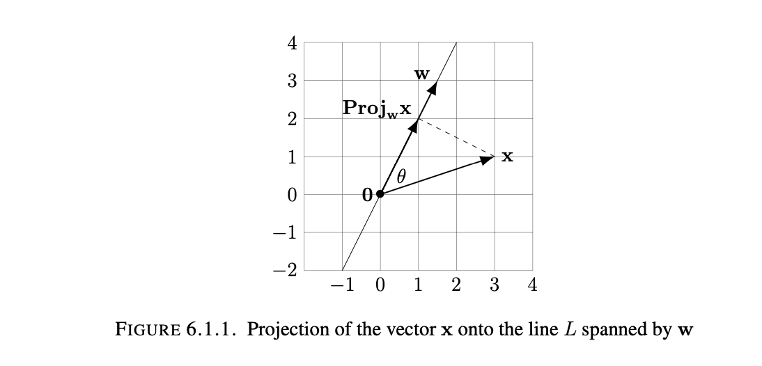
Algebraic Method: We look for a scalar c for which x-cw is orthogonal to every vector in L. The points of L=span(w) are those of the form aw for scalars a, so we seek c making $(x-cw)\cdot{aw}=0$ for every scalar a. The dot product has the property $(x-cw)\cdot{(aw)}=a((x-cw)\cdot{w})$, so actually all we need to do is make sure that $(x-cw)\cdot{w}=0$. We can rewrite this dot product as $0=(x-cw)\cdot{w}=x\cdot{w}-(cw)\cdot{w}$. This can further be rearranged as $c(w\cdot{w})=x\cdot{w}$. Since w is not a zero vector, we can rearrange into the final form: $c=\frac{x\cdot{w}}{w\cdot{w}}$. This is all to find the scalar that minimizes the distance between the linear subspace and the point, but we can go further and express it as a vector to make a more comprehensible output in terms of some vector v. $$v=\frac{x\cdot{w}}{w\cdot{w}}w$$

Geometric Method: I will not go too into depth since this method cannot be generalized to larger Rn(which is what we really care about). Essentially it revolves around making an acute angle $\theta$ between line L and the vector describing point x and using the alternative way of describing the dot product in terms of cosine and the magnitude of the two vectors to find that the projection can be expressed as: $(||x||cos{\theta})\frac{w}{||w||}$.

Proposition 6.1.1: Let $L=span(w)={cw : c \in R}$ be a 1-dimensional linear subspace of Rn(so w is not equal to 0), a “line”. Choose any point $x \in \mathbf{R}^n$. There is exactly one point in L closest to x, and it is given by the scalar multiple $$\frac{x\cdot{w}}{w\cdot{w}}w$$ of w. This is called “the projection of x into span(w)”; we denote it by the symbol $Proj_{w}(x)$.

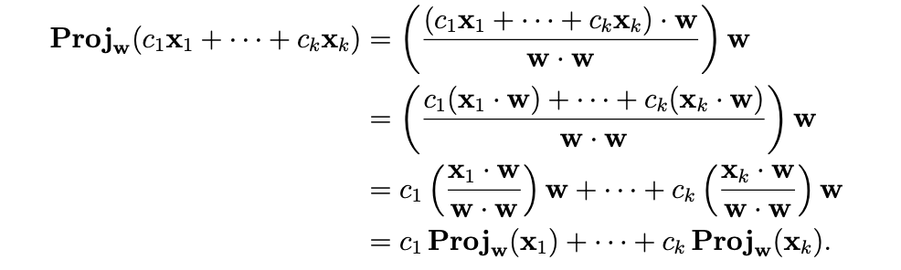
We can find a faster way to project multiple points onto one line. The key observation in doing so is that the formula for the $Proj_{w}(x)$ behaves well for any linear combination of n-vectors $x_1, x_2, …, x_k$: the projection of a linear combination of all the $x_i$’s is equal to the corresponding linear combination of the projections.

Example 6.1.4: Sometimes it is useful(much more so in subsequent sections) to express a projection onto a vector which is a linear combination. Right below here I have included an interesting property that arises out of the linear properties of the dot product. Basically it just shows us that we can split up a projection into a combination of projections onto separate vectors.

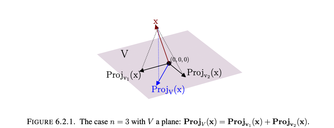
Now we will move onto projecting onto a general subspace. Essentially we will just be finding the point in a linear subspace V of Rn nearest to a chose $x\in\mathbf{R}^n$, which we denote as $Proj_{V}(x) \in V$. This nearest point to x will be, as mentioned earlier computed as a sum of projections onto x into lines through 0 in V arising from an orthogonal basis of V.

Essentially we need to find some vector $v$ that can be expressed as some linear combination of the other orthogonal basis vectors. Dotting this vector $v$ with $x-Proj_{V}(x)$(this is also perpendicular to everything in V) will yield 0, and we will be able to prove that this vector is indeed the closest vector to the point x.

Theorem 6.2.1: (Orthogonal Projection theorem version I) For any $x\in\mathbf{R}^n$ and linear subspace V of $\mathbf{R}^n$, there is a unique v in V closest to x. (In symbols, $||x-v||<||x-v’||$ for all $v’$ in V with $v’\neq{v}$). This v is called the Projection of x onto V, and is denoted $Proj_{v}(x)$. The projection $Proj_{v}(x)$ is also the only vector $v \in V$ with the property that the displacement $x-v$ is perpendicular to V. If V is nonzero then for any orthogonal basis $v_1, v_2, …, v_k$ of V we have $$Proj_{V}(x)=Proj_{v_1}(x)+Proj_{v_2}(x)+…+Proj_{v_k}(x)$$, where $Proj_{v_i}(x)=\frac{(x\cdot{v_i})}{(v_{i}\cdot{v_i})}v_i$.

(For $x\in V$ we have $Proj_{V}(x)=x$–the point in V closest to x is itself.)

It may seem confusing that the basis must be orthogonal for this formula to hold true, afterall we have proved that for linearly independent vectors, we can represent any vector in their span by some linear combination of those vectors. This is still true, but the issue is that when we are projecting onto two non-orthogonal vectors, there will be redundancy in the projections. Imagine two very close vectors v and w representing some linear subspace V, when we take the projection of some point x onto V, these projections will basically be the same if they are very close. So when it comes to adding these projections to find the vector y that represents x’s projection, we will be way off due to the overlap which v and w shared. Thus, it is essential that we always ensure that we have an orthogonal basis when projecting onto some linear subspace as it will ensure there is zero redundancy in the projections.

Theorem 6.2.4(Orthogonal Projection Theorem, Version II): (Orthogonal Projection Theorem, Version II). If V is a linear subspace of $\mathbf{R}^n$ then every vector $x\in \mathbf{R}^n$ can be uniquely expressed as a sum $$x=v+v’$$ with $v\in V$ and $v’$ orthogonal to everything in V. Explicitly, $$v=Proj_{V}(x)$$ and $$v’=x-Proj_{v}(x)$$.

^ My preferred way of looking at this theorem.

How to find an orthogonal basis for $V\in \mathbf{R}^n$: We know how to find a projection onto a general subspace V, but to do so we must have an orthogonal basis for the linear subspace V. This will be addressed in chapter 19 and 20 using the Gram-Schmidt process and some matrix algebra.

Maybe include proof 6.3

Chapter 7

Applications of Projections in $\mathbf{R}^n$: orthogonal bases of planes and linear regression

So far we have found a formula for projection to a linear subspace of $\mathbf{R}^n$ using an orthogonal basis of the linear subspace, but we can also go the other way and use projections to find an orthogonal basis for a linear subspace.

Theorem 7.1.1: Suppose $x$, $y$ $\in \mathbf{R}^n$ are nonzero, and not scalar multiples of each other. The vectors y and $x’=x-Proj_{y}(x)$ constitute an orthogonal basis of span(x,y).

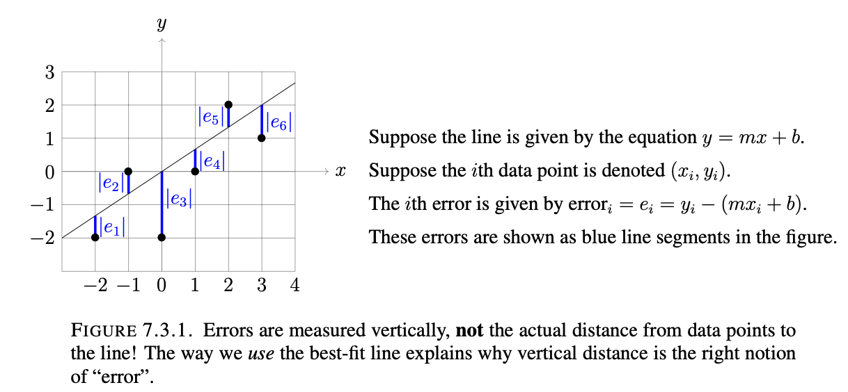
Fitting a function to data: Essentially we want to find the function $f(x) = mx + b$ that “best fits” n data points $(x_1,y_1),…,(x_n,y_n)$. We just want to make some $f(x_i)$ to be as close as possible to $y_i$ for i. The error: $error_i=y_i-(mx_i+b)$ measures in absolute value how close the line $y=mx+b$ is vertically to $(x_i,y_i)$. Since we are arbitrarily measuring the “best fit” we can square the error for each i and find the sum of errors of the set (x, y). $\sum_{i=1}^n(y_i-(mx_i+b))^2$.

Example 7.3.2

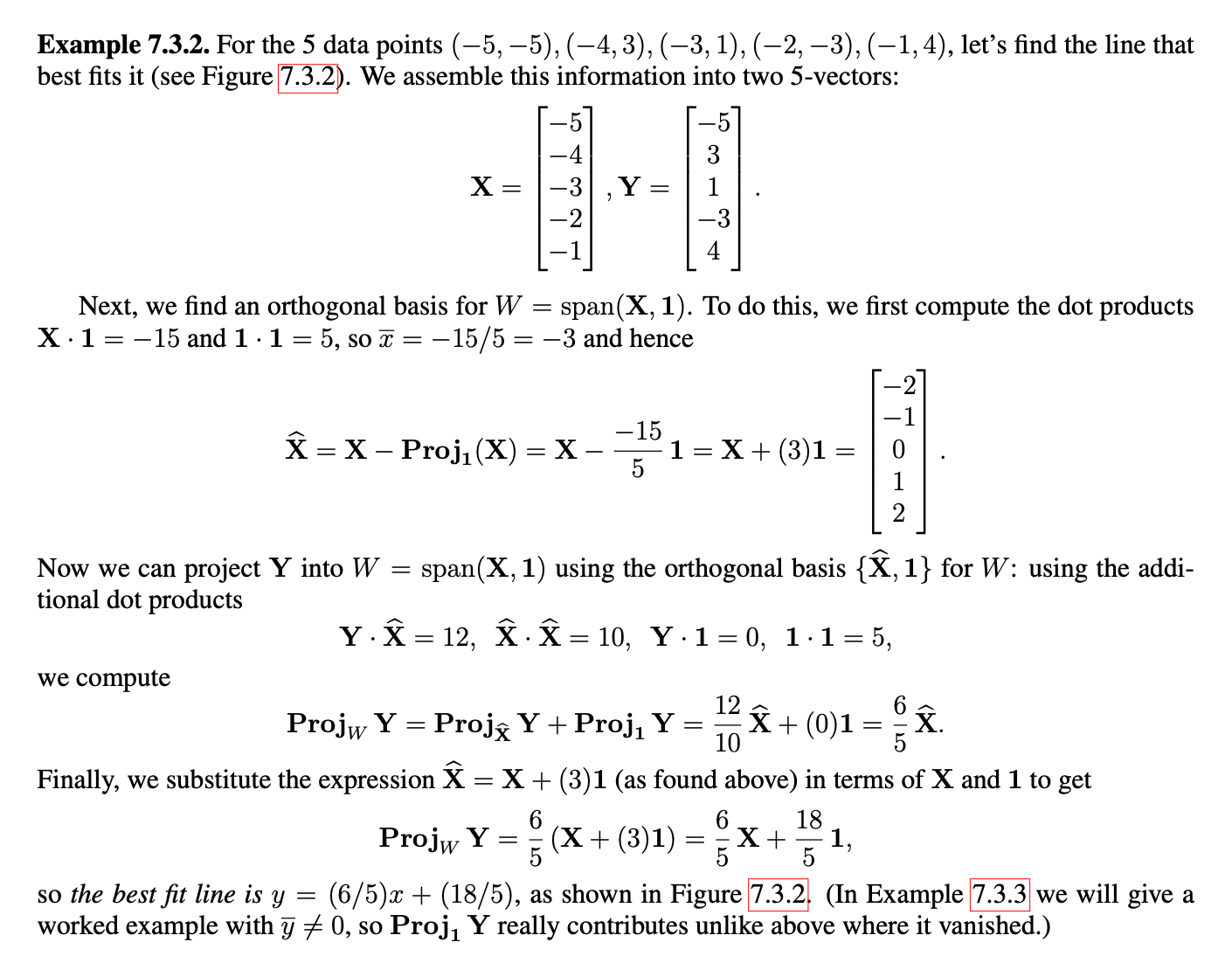
General 7.3: Here is the general method. Suppose we are given n data points $(x_i, y_i)$ that do not lie on a common vertical line. To find the best line $y=mx+b$, do the following. (i)Assemble the given data into two n-vectors $$X=\begin{bmatrix} x_1 \\ \vdots \\ x_n \end{bmatrix}$$ & $$Y=\begin{bmatrix} y_1 \\ \vdots \\ y_n \end{bmatrix}$$. Also let 1 be the n-vector all of whose entries are equal to 1

(ii) For $W=span(X,1)$, we will compute $Proj_w(Y)$ as a linear combination of $mX+b$1 of X and 1; those coefficients are exactly the coefficients of the best line $y=mx+b$.

(iii) To compute $Proj_W(Y)$, use the orthogonal basis 1 and $\hat{X}=X-Proj_1(X)$ for W. Explicitly $$\hat{X}=\begin{bmatrix} x_1-\bar{x} \\ \vdots \\ x_n-\bar{x} \end{bmatrix}$$ and so $Proj_{W}(Y)$=$(\frac{Y\cdot{\hat{X}}}{\hat{X}\cdot{\hat{X}}})(\hat{X})$ + $\bar{y}1$ $=$ $(\frac{Y\cdot{\hat{X}}}{\hat{X}\cdot{\hat{X}}})(X-\bar{x}1)+\bar{y}1$

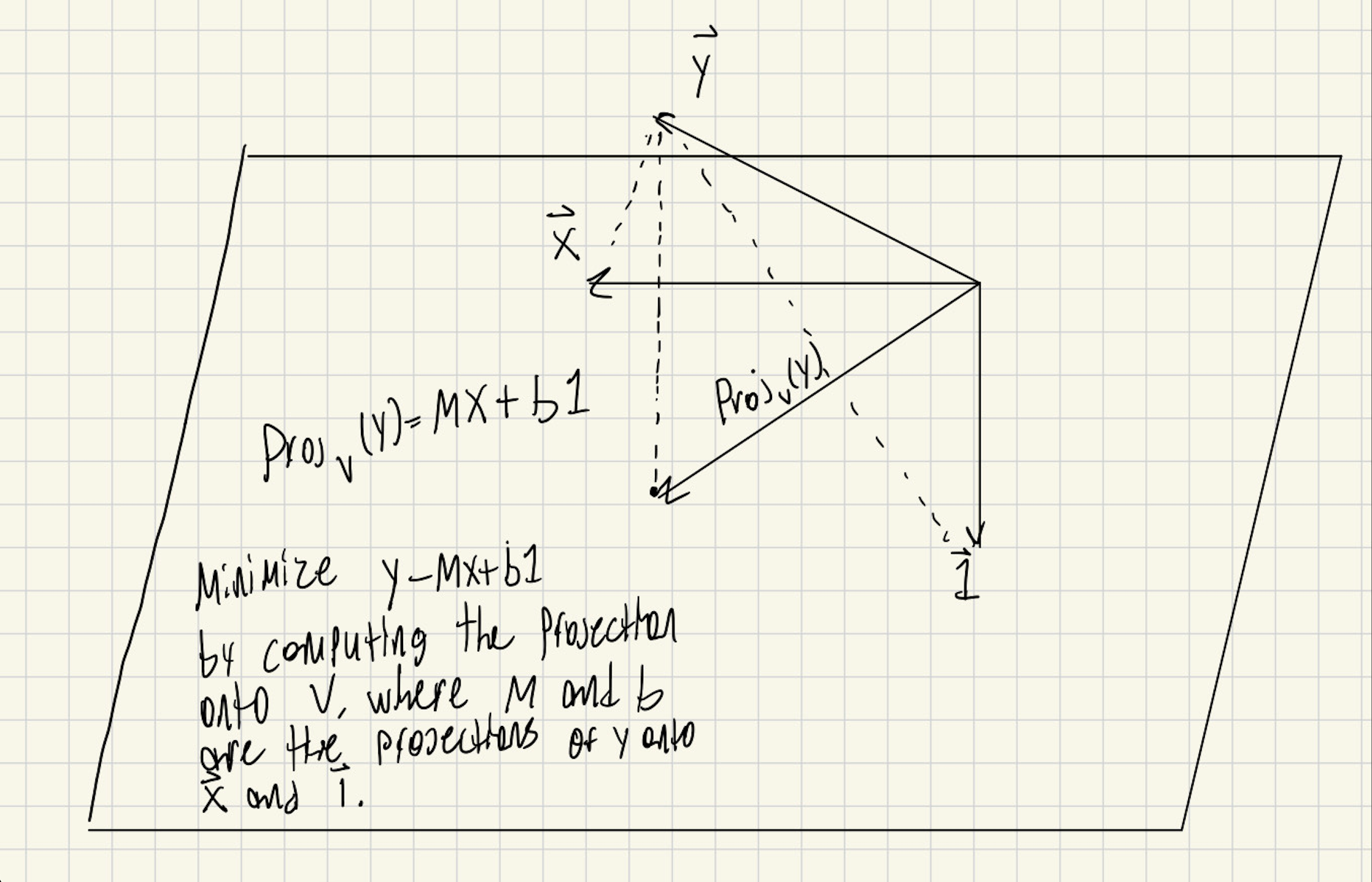
If we imagine minimizing this error between the data points given by the vector Y and the line of best fit defined by mX+b in terms of $\mathbf{R}^n$, then we can interpret this formula as finding the projection(point of minimal distance between it and linear subspace V) of Y onto the linear subspace defined by X and 1. Here is an image to help:

Whenever $\bar{x}=0$ we have $\hat{X}=X$.

if $\bar{x}=0$ then $Proj_{W}(Y)=(\frac{Y\cdot{X}}{X\cdot{X}})X+\bar{y}1$, so $m=(\frac{Y\cdot{X}}{X\cdot{X}})$ and $b=\bar{y}$ whenever $\bar{x}=0$. Only when $\bar{x}=0$!!!!

Finding the distance between two lines: Let $l_1$ be the line in $\mathbf{R}^3$ that is parallel to $v=\begin{bmatrix} 2 \\ 3 \\ 4 \end{bmatrix}$ and goes through $a=\begin{bmatrix} 1 \\ 0 \\ 0 \end{bmatrix}$, and let $l_2$ be the line in $\mathbf{R}^3$ that is parallel to $v=\begin{bmatrix} 4 \\ 3 \\ 2 \end{bmatrix}$ and goes through $b=\begin{bmatrix} 0 \\ 1 \\ 0 \end{bmatrix}$. What is the closest distance between $l_1$ and $l_2$?

Here is an image to help with illustration:

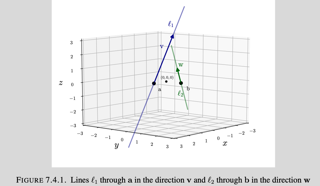
To solve this problem, we can express the solution as finding a closest point to a plane(projection). The parametric form of lines in space gives $l_1$ consists of the points of the form $a+tv$ for an arbitrary scalar $t$, and $l_2$ consists of the points of the form $b+t’w$ for an arbitrary scalar $t’$. The distance between any two points on the lines can be provided by $||(a+tv)-(b+t’w)||$. We look for $t$ and $t’$ that minimize this distance.

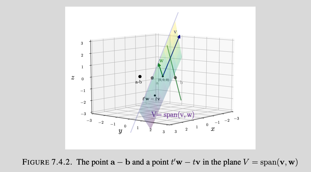
Instead of trying to arbitrarily search for a scalar that minimizes the distance between these lines, we can instead re-write the form for the distance between any two points in the line as: $(a+tv)-(b+t’w)=(a-b)-(t’w-tv)$, which we can interpret as the distance between the vector/point $a-b$ and the vector $t’w-tv$. Varying $t$ and $t’$ gives thew span of the vectors $v$ and $w$. This now offers us the alternative geometric interpretation of the problem included below:

We can clean up this to produce a more familiar image of a projection onto a linear subspace V:

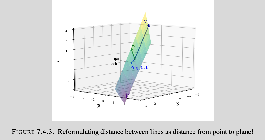
I personally would not have arrived at this creative reinterpretation of the problem, but now we can see the intuition behind this reinterpretation.

Step 1: We want to use a projection onto a linear subspace to minimize the distance between the point and the linear subspace V defined by the span of vectors v and w. To do this we need to have an orthogonal basis for the subspace we want to project on, so we compute $v’=v-Proj_{w}(v)=v-\frac{v\cdot{w}}{w\cdot{w}}w$.

Step 2: We will then compute the projection onto the linear subspace defined by v’ and w: $Proj_{V}(a-b)=\frac{(a-b)\cdot{w}}{w\cdot{w}}w + \frac{(a-b)\cdot{v’}}{v’\cdot{v’}}v’ = cw + c’v'$

Step 3: Now we have this arbitrary projection in terms of unfamiliar terms, so we must translate it back into $v$ and $w$, so that we can find what parameters $t$ and $t’$ minimize the distance between the lines. We can do this by re-writing v’ as $v-Proj_{w}(v)=v-\frac{v\cdot{w}}{w\cdot{w}}w$. After doing this we should end up with some linear combination of v and w. We know that the distance between lines was expressed as $(a-b)-(t’w-tv)$, so we can find the scalars $t$ and $t’$ by equating $(t’w-tv)$ to our linear combination obtained above.

Final Step: Plug $t$ and $t’$ back into the original equations of both of the lines to get two vectors then find the magnitude of the vector between those two vectors.

Chapter 8

Multivariable functions, level sets, and contour plots

This is where the class begins a slight detour into multivariable calculus before ultimately finishing up the content of linear algebra. Keep in mind the notes for this class are supposed to encapsulate optimization in any space, so coupling linear algebra with a bit of multivariable calculus is a very logical thing to do.

To begin we will talk about the different types of multivariable functions.

Definition 8.1.1: A scalar-valued function is a function $\mathbf{R}^n$->$R$ (that is to say, with m=1). In other words, a scalar valued function gives real number outputs.

Generally any function which takes multiple inputs and incorporates them in a single expression is going to be a scalar valued function, since it will(likely) have a single 1-dimensional output.

Definition 8.1.7: A vector-valued function is a function f: $\mathbf{R}^n$->$\mathbf{R}^m$ with general $m \geq 1$. In other words, a vector valued function gives output considered as vectors in some $\mathbf{R}^m$.

A vector valued function f: $\mathbf{R}^n$->$\mathbf{R}^m$ can be expressed in terms of $m$ scalar-valued component functions or coordinate functions $f_1,…,f_m:\mathbf{R}^n$->$R$, defined by the expressions

$$f(x)=\begin{bmatrix} f_{1}(x) \\ \vdots \\ f_{m}(x) \end{bmatrix}=(f_{1}(x),…,f_{m}(x))$$

(depending on whether we consider the output to be a “vector” or a “point”), with each $f_j$ a scalar-valued function. We can write the output of f on the input $x\in \mathbf{R}^n$ in at least three ways: $$f(x)=f(\begin{bmatrix} x_1 \\ \vdots \\ x_n \end{bmatrix})=f(x_1,…,x_n)$$, depending on whether we want to keep things compact, emphasize that the inputs to f is considered as a vector in $\mathbf{R}^n$, or emphasize that the output of f depends on n real-number inputs(coordinates of vector x).

We can also compose certain compatible multivariable functions(meaning that given certain parameters, we can first evaluate the output of the first function, then input that output into the second function as new parameters).

Definition 8.2.2: If g$:\mathbf{R}^n$->$\mathbf{R}^p$ and f$: \mathbf{R}^p$->$\mathbf{R}^m$ are multivariable functions (note that g has output belonging to $\mathbf{R}^p$ on which f is applied), we can form a new composite function:

Take an input(x) in $\mathbf{R}^n$; first apply g to it, and then apply f: $$x \in \mathbf{R}^n \leadsto^{g} \mathbf{R}^p \leadsto^{f} \mathbf{R}^m$$

As a shorthand, we write this new function as $f\circ{g}$; the symbol $\circ$ is read as “composed with.” In symbols, new function is given by:

$(f\circ{g})(x)$=($f$ applied to $g(x))=f(g(x))$

Order of composition matters!!! If you are given g which goes from n=3 to p=1 and f which goes from p=1 to m=2: It works one way since 3–>1–>1–>2 is a totally fine order of composition, but it doesn’t work the other way since 1–>2–>x–>3–>1. Since the intermediary vectors dimensions don’t match up the composition is impossible.

Here’s an example of a graph of a composed function:

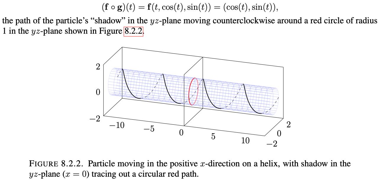
Now how can we visualize these multivariable functions? Since dealing with multiple variables introduces many more layers of complication with visualization, we have multiple ways to think graphically about these multivariable functions. The first way is through an actual graph in which we plot out the inputs on separate axis and make an additional axis for the output. The second way we can visualize them is by looking at their contour plots, that is to say, we look at cross sections of the output graph.

Definition 8.3.1: The graph of $f:\mathbf{R}^n$->$R$ is the subset of $\mathbf{R}^(n+1)$ (not $\mathbf{R}^n$) defined as:

Graph$(f)={(x_1,…,x_n,z) \in \mathbf{R}^{n+1}:z=f(x_1,…,x_n)}$.

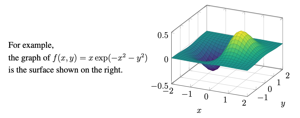
Here’s a couple images to help:

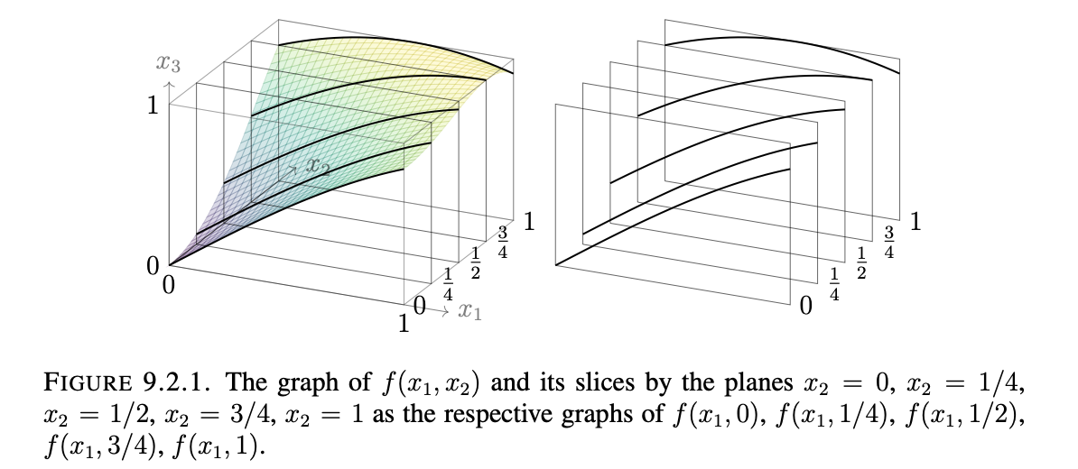
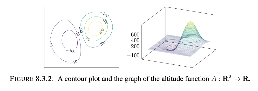
Definition 8.3.4: Let $f:\mathbf{R}^n$->$R$ be a function. For any $c \in R$, the level set of f at level c, is the set of points $(x_1,…,x_n) \in \mathbf{R}^n$ for which $f(x_1,…,x_n)=c$ It is also called the c-level set of f.

If $f$ is a function $\mathbf{R}^2$->$R$ of 2 variables then a contour plot of $f$ is a picture in $\mathbf{R}^2$ that depicts the levels sets of $f$ for many different values of c (often with some common difference for consecutive level sets, such as common difference of 10, 4, 1, or 0.5).

Here’s an example of a contour plot of a function and its graph:

When you are given a specific set S defined in 3D space (R³) by an equation, the only functions f and h that will have S as their common zero level set are those functions that incorporate the exact same equation.

Here’s the reasoning behind this:

The set S is defined by an equation in the form: S = {(x, y, z) ∈ R³ : F(x, y, z) = 0}

Where F(x, y, z) is some multi-variable function of x, y, and z.

For functions f and h to have S as their common zero level set, it means: f(x, y, z) = 0 AND h(x, y, z) = 0 must both be true exactly when F(x, y, z) = 0.

In other words, the functions f and h must incorporate all the same terms and operations as the original function F that defines the set S.

Let’s use an example to illustrate this further:

Suppose the set S is defined by the equation: S = {(x, y, z) ∈ R³ : x² + 3y - 2z = 0}

Then the only valid functions f and h that would have S as their common zero level set would be:

f(x, y, z) = x² + 3y - 2z h(x, y, z) = x² + 3y - 2z

Any other functions, even if they share some terms with the original equation, would not result in the same zero level set as S.

For example, a function like: f(x, y, z) = x² + 3y h(x, y, z) = -2z

would not work, because their zero level sets would not coincide with the original set S.

The key point is that the functions f and h must incorporate the exact same equation as the one defining the original set S in order for their zero level sets to perfectly match.

Clean up these insights and include notes from class. Also include a few examples and images.

Chapter 9

Partial derivatives and contour plots

To understand the derivatives of multivariable functions, it is useful to revisit single-variable derivatives. The main interpretations for the derivative in single variable calculus have been included below:

(i) A basic interpretation of the derivative is that it represents the ‘instantaneous rate of change’. If we change the value of x slightly from x=c to something very close to that point, say c+0.00001, then the derivative provides a good approximation of how much $f(x)$ changes. Indeed, $f’(c)$ is approximately the ratio of change of output to the (small) change in input near x=c. So if we increase c to c+0.00001, then to a good degree of approximation, the value of $f$ has changed from $f(c)$ to $f(c) + f’(c)(0.00001)$. In general we can represent this small change in x as h and we can express the value of the expression $f(c+h)$ as $f’(c)h$, or equivalently $f(x)\approx f(c) + f’(c)(x-c)$ for x near c.

(ii) The number $f’(c)$ is the slope of the line tangent to the graph at the point $(c,f(c))$.

Limit definition of single-variable derivative: $$f’(c)=\lim_{h \to 0}\frac{f(c+h)-f(c)}{h}$$

Somewhat important note to think about: It is easy to get drawn into thinking that these formulas for f′(x) for familiar functions f(x) are all that derivatives are, but they are simply the outcome of specific calculations which are ultimately deduced from the limit definition. -courtesy of the textbook :)

Recall that for single-variable functions, we can use the derivative as a marker for extrema(i.e. when the derivative is zero, it indicates that there is a max/min since the function is neither increasing or decreasing at these points). In these cases we find where the first derivative is zero then we determine whether it is a max, min, or point of inflection using either a plug in method or by using the second derivative to se whether the function has a positive or negative rate of change(or 0 if its a point of inflection).

That’s enough of talking about single-variable functions.

Consider a function $f(x_1,x_2)$. Just like single-variable functions we can leverage the concepts of derivatives to find some instantaneous rate of change for the function. Unlike single-variable functions, however, the derivative in this setting can have many more meanings, as there are many independent variables. Multivariable calculus uses partial derivatives to articulate change in a more precise way. Later on other ideas such as directional derivatives, the gradient, and the derivative matrix will provide more precise means to approximate the point $f(x_1,x_2)$ near (a,b) with a linear function.

The main idea of partial derivatives is to treat multivariable functions as collections of functions of one variable, treating the other variables in each case as constants.

Definition 9.2.2: The partial derivative of f with respect to $x_1$ at the point (a,b), denoted in any of the equivalent ways included below means the derivative of the function $f(x_1,b)$ at $x_1=a$.

$\frac{\partial f}{\partial {x_1}}(a,b), f_{x_1}(a,b)$ There’s another way, but the markdown for it is just inefficient and it’s scarcely used so I won’t include it here.

Another way to phrase it is that the partial derivative of $f$ with respect to $x_1$ at $(a,b)$ is the instantaneous rate of change of $f$ at the point $(a,b)$ if we only move in the $x_1$ direction (so $x_2$ is held constant, at the value b). The formal definition is once again as a limit of difference quotients: $$\frac{\partial f}{\partial {x_1}}(a,b)=\lim_{h \to 0}\frac{f(a+h,b)-f(a,b)}{h}$$.

Note that this works the exact same for $x_2$ just need to hold $x_1$ constant. Actually the same applies for any $x_i$ so long as all other $x_j$ are held constant.

When computing partial derivatives think of the $x_j$’s for $j \neq i$ as constant(don’t input any value) and apply the single-variable differentiation rules in terms of $x_i$ to obtain the new function of n variables, $f_{x_i}(x_1,…,x_n)$. Then substitute for the other terms.

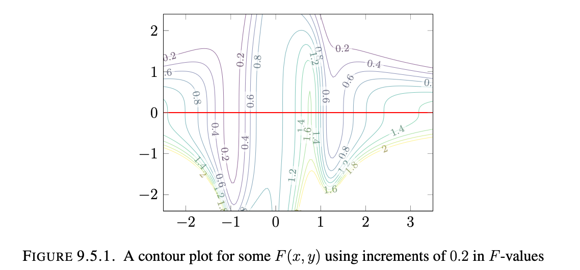
Partial derivatives discussed visually: Contour plots can be used to gather qualitative data about a multivariate function. We can proces information about the partial derivatives of a function by taking one of the variables and setting it to a constant value, then tracing out a path across the level sets. The frequency of crossing corresponds to the magnitude of the partial derivative and the sign of the second derivative(if the contour labels are increasing at a positive or negative rate.

Here are a few examples of contour plots which we can look at to discuss more of the qualities of these multivariable functions:

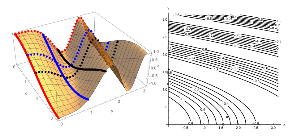
Formally: Visualize $F(x,y)$ as the height above $(x,y)$ on the surface of the graph $z=F(x,y)$ on the curve in the surface graph $z=F(x,y)$, where x is the east-west coordinate and yu is the north-south coordinate. Then:

-$\frac{\partial F}{\partial {x}}(a,b)$ equals the slope experienced by someone walking on the surface just as they go past the point $(a,b)$ from west to east.

-$\frac{\partial F}{\partial {y}}(a,b)$ equals the slope experienced by someone walking on the surface just as they go past the point $(a,b)$ from south to north.

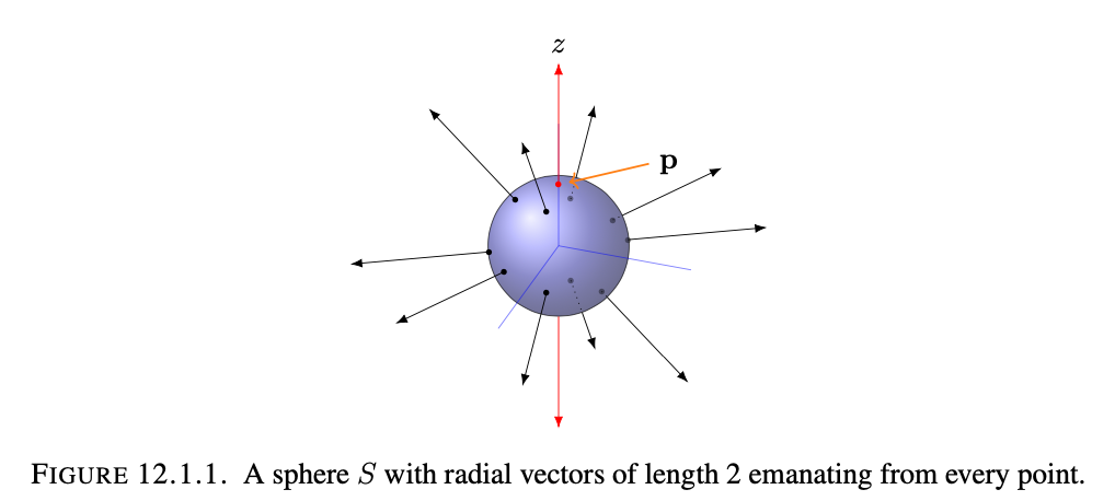
On a contour plot of the function $F(x,y)$, the partial derivatives can be interpreted as follows:

-The sign of $\frac{\partial F}{\partial {x}}(a,b)$ tells us whether the labels of the contours (which represent the values of $F$) are increasing or decreasing as we walk through $(a,b)$ form west to east.

-The sign of $\frac{\partial F}{\partial {y}}(a,b)$ tells us whether the values of $F$ on the contours are increasing or decreasing as we walk through $(a,b)$ from south to north.

-If $\frac{\partial F}{\partial {x}}(a_1,b_1) \geq \frac{\partial F}{\partial {x}}(a_2,b_2) \geq 0$ then in the x-direction the slope at $(a_1,b_1)$ is steeper than the slope at $(a_2,b_2)$, so the contours (when shown for uniform increments in $F$-values) are spaced closer together as we move east across $(a_1,b_1)$ than they are as we move east across $(a_2,b_2)$. There is a corresponding statement for negative x-partial derivatives(still moving east). Same could also be said for $\frac{\partial F}{\partial {y}}$ moving north.

We can practice these concepts of partial derivatives on contour plots here:

Definition 9.6.3: For a function $f(x_1,…,x_n)$ of n variables that is differentiable in each $x_i$ separately, the second partial derivatives are defined to be:

$\frac{\partial^2 F}{\partial {x_i}\partial {x_j}}$=$x_i$-partial derivative of $\frac{\partial F}{\partial {x_j}}$ (when j=i it is denoted $\frac{\partial^2 F}{\partial {x_i}^2}$)

Theorem 9.6.4: (Clairaut-Schwarz). Consider a function $f(x_1,…,x_n)$ that is continuous, and for $1 \geq i,j \leq n$ suppose that the partial derivatives $\frac{\partial F}{\partial {x_i}}$ and $\frac{\partial F}{\partial {x_j}}$ as well as the second partial derivatives $\frac{\partial^2 F}{\partial {x_i}\partial {x_j}}$ and $\frac{\partial^2 F}{\partial {x_j}\partial {x_i}}$ exist and are continuous. Then the order of applying $\frac{\partial}{\partial{x_i}}$ and $\frac{\partial}{\partial{x_j}}$ to $f$ doesn’t matter:

$\frac{\partial^2 F}{\partial {x_i}\partial {x_j}} = \frac{\partial^2 F}{\partial {x_j}\partial {x_i}}$

Chapter 10

Maxima, minima, and critical points

With functions of multiple variables we need to define what it means for a function f: Rn->R to have a local maximum or a local minimum. We can generalize this but for now I will include the definition for a function of 2 variables.

Definition 10.2.1: A function $f(x,y)$ achieves a local maximum at (a,b) if $f(a,b) \geq f(x,y)$ for all (x,y) which are sufficiently near (a,b). (i.e. moving in any direction will decrease f)

A function $f(x,y)$ achieves a local minimum at (a,b) if $f(a,b) \leq f(x,y)$ for all (x,y) which are sufficiently near (a,b). (i.e. moving in any direction will increase f)

Theorem 10.2.2: Suppose that a point $a \in \mathbf{R}^n$ is either a local maximum or a local maximum of $f$. Then all partials derivatives of $f$ vanish at $x=a$; i.e., $\frac{\partial F}{\partial {x_i}}(a)=0$ for $1 \leq i \leq n$.

Definition 10.2.3: If $\frac{\partial F}{\partial {x_i}}(a)=0$ for all $1 \leq i \leq n$ then we say a is a critical point for $f$. In particular, every local maximum and every local minimum of $f$: $\mathbf{R}^n$->$R$ is a critical point.

Include some examples here

We emphasize that if a is a critical point of $f$: $\mathbf{R}^n$->$R$, then it may be neither a local maximum nor a local minimum. In fact, for functions of two or more variables there is a new phenomenon:

Definition 10.2.10: A critical point $a \in \mathbf{R}^n$ of $\mathbf{R}^n$->$R$ is a saddle point if (i) as we move away from $a$ along some line, then $f$ increases nearby, so $a$ is a local minimum along that line, and (ii) as we move away from $a$ along some other line then $f$ decreases, so $a$ is a local maximum along that line.

Such behavior can happen with n variables when n > 1 because then there are “more lines” in Rn through a point along which we can move away from the point: in R there is only one line through a point, but in R2 there are many lines through a point (e.g., not only horizontal, but also vertical, diagonal, etc.), let alone in Rn for n>2. This is a genuinely multivariable phenomenon.

Example problem

Extrema on Boundaries: Oftentimes we will want to find the maximum, minimum points of a function over a restricted domain. In these cases we will have to evaluate the extrema of the function computed by solving $f_x=f_y=0$ along with solving what the maximum and minimum points are of the curves(in 3 space) defined by the intersection of $f$ with the boundaries. For these cases we simply plug in the restricting equations(of the boundary) into $f$ for each boundary side/curve, then we find what the extrema are of that restricted function. Then we compare these results with the local extrema.

Theorem 10.4.6: For a function $f$: $\mathbf{R}^n$->$R$ and a region D inside $\mathbf{R}^n$, suppose the function $f$: D->$R$ considered on D has a local extremum at a point $a \in D$ (i.e. $f(x) \leq f(a)$ for all $x \in D$ near a, or $f(x) \geq f(a)$ for all $x \in D$ near a).

The point $a$ must be a critical point of $f$ when $a$ is in the interior of D. In particular, any local extrema of $f$ : $D$->$R$ either is a critical point on the interior of D or is a boundary point of D.

Sometimes these systems of equations that we set up for solving for extrema can be extremely challenging. While we will learn techniques later that will help reduce the difficulty of these problems for now I will offer a few tips.

(i) This is obvious but start with the simplest of your equations. If your condition for $f_x$ looks easy to factor and find values that give $f_x=0$ then start with that!

(ii) If the equations that give the conditions for the partials to be equal to zero are linear, then just treat it as any other linear system of equations solved earlier.

(iii) Oftentimes there will be many variables to solve for. In these cases trying to work with substitution isn’t a bad idea.

(iii) Once you have some conditions that must be met for certain partials to be zero, start checking how those conditions restrict other equations. MAKE SURE TO CHECK ALL CONDITIONS! Sometimes there will be redundancy, but checking is better than forgetting a critical point.

(iv) This more or less goes with what I just stated but there will be paths created by each restriction. FOLLOW EVERY SINGLE PATH!

(v) Once you obtain all the critical points–just double check they make sense.

Chapter 11

Gradients, local approximations, and gradient descent!

We now know how to approximate the value of a multivariable function and how to find the extrema, all using partial derivatives. But now we seek to generalize the idea of derivatives of multivariable functions. We can do this by essentially packaging all the partial derivative information into a vector valued function called the gradient(denoted $\nabla f$).

*Little note We will sometimes write the inputs as vectors; e.g. when n = 2 think of $f$ as a function of the x,y vector.

Definition 11.1.1: Consider a function $f$: $\mathbf{R}^n$->$R$.

The gradient of $f$ is defined to be: $$\nabla f= \begin{bmatrix} \frac{\partial f}{\partial {x_1}} \\ \frac{\partial f}{\partial {x_2}} \\ \vdots \\ \frac{\partial f}{\partial {x_n}} \end{bmatrix} $$.

Note that the gradient is an n-vector. For $x$ near $a \in \mathbf{R}^n$, the linear approximation to $f$ is $f(x) \approx f(a) + ((\nabla f)(a)) \cdot (x-a)$.

This looks like the single variable case, but now we account for each variable and evaluate using the dot product to sum the products of each partial derivative with their respective small change $(x_i-a_i)$.

Note that the approximation is very accurate when hand kare very small.

Theorem 11.2.1: Let $f$: $\mathbf{R}^2$->$R$ be a scalar valued function, and suppose $(\nabla f)(a,b) \neq 0$.

(i)The gradient $(\nabla f)(a,b)$ is perpendicular to the level set of $f$ that goes through $(a,b)$. It points in the direction of maximal increase for $f(x,y)$ for $(x,y)$ moving away from $(a,b)$. The following figure demonstrates this with the function $f(x,y)=xy-x$:

(ii) The equation $(\nabla f)(a,b) \cdot \begin{bmatrix} x-a \\ y-b \end{bmatrix}=0$ in the $(x,y)$ plane is the line tangent to the curve in the contour plot of $f(x,y$ through $(x,y)=(a,b)$. Explicitly, the equation of this line is $f_x(a,b)(x-a)+f_y(a,b)(y-b)=0$.

Theorem 11.2.2: For a scalar valued function $f$: $\mathbf{R}^3$->$R$ and a point a for which $(\nabla f)(a) \neq 0$, the gradient vector is perpendicular to the plane tangent to the level set opf $f$ through a. In particular, this tangent plane has the equation $(\nabla f)(a_1,a_2,a_3) \cdot \begin{bmatrix} x-a_1 \\ y-a_2 \\ z-a_3 \end{bmatrix}=0$.

Include some examples if time is provided

Gradient Descent: The main reason I’m interested in studying multivariable calculus is to optimize functions of n variables. Realistically if we were to set up such a problem for large n, we couldn’t really hope to find an exact solution, however with the help of gradient descent we can get a very good numerical approximation. The textbook has a really great analogy that I’ll include here which helps to explain the process of gradient descent.

“Imagine that a raindrop falls on a hill. It will head to the bottom – water always finds the lowest elevation. Or at the very least it will find a local minimum: it might not find the bottom of the hill, but it will find a lake halfway down the hull, perhaps. The raindrop certainly doesn’t know anything about the geography of the hill. However, at every moment, it simply ‘chooses’ to roll in the steepest possible direction. It is not only the raindrops that find local minima. Physical systems find energy minima, and they do so by moving in the ‘direction’ where potential energy decreases the most. Essentially, to find the minimum of a function, travel in the direction in which $f$ decreases the fastest. And do the opposite to find it’s maximum.”

But how do we find the direction of maximum increase or decrease?

Essentially we want to find the vector, that when we travel on $f$ in its direction, $f$’s value increases/decreases the most. To find how much $f$ changes in a particular direction, all we have to do is find $(\nabla f) \cdot v$ where $v$ is a unit vector. This just sums up how much $f$ changes when it travels a certain amount a, b (components of $v$–just using \mathbf{R}^2 here for simplicity) in each direction.

To test how fast $f$ is increasing or decreasing in the direction of $v$ we use local approximation: $f(a+tv) \approx f(a) + (\nabla f)(a) \cdot (tv) = f(a) + t(\nabla f)(a) \cdot v$. This says that if we move a small distance $|t|$ in the direction $v$ for $t>0$ and in the direction of $-v$ for $t<0$ then the change in $f$ is $\approx t((\nabla f)(a)\cdot v)$, whose rate of change with respect to $t$ is $(\nabla f)(a) \cdot v$.

Now we can use geometry to chose the unit vector $v$ such that this change with respect to $t$ is largest. Recall the dot product formula but apply our new vectors: $(\nabla f)(a)=||(\nabla f)(a)||||v||\cos{\theta}$. Clearly the dot product, which represents the rate of change, is most positive when the angle between the vectors is 0, and most negative when the angle between the vectors is 180. This provides us with the following theorem:

Theorem 11.3.2: Let $f$: $\mathbf{R}^2$->$R$ be a scalar valued function and $a \in \mathbf{R}^n$ a point where the gradient is nonzero.

The gradient at a, or rather the associated unit vector $(\nabla f)(a)/||(\nabla)(a)||$, is the direction in which $f$ increases most rapidly, and its negative is the direction in which $f$ decreases most rapidly at $a$.

To demonstrate this process I have just provided the following example from the text:

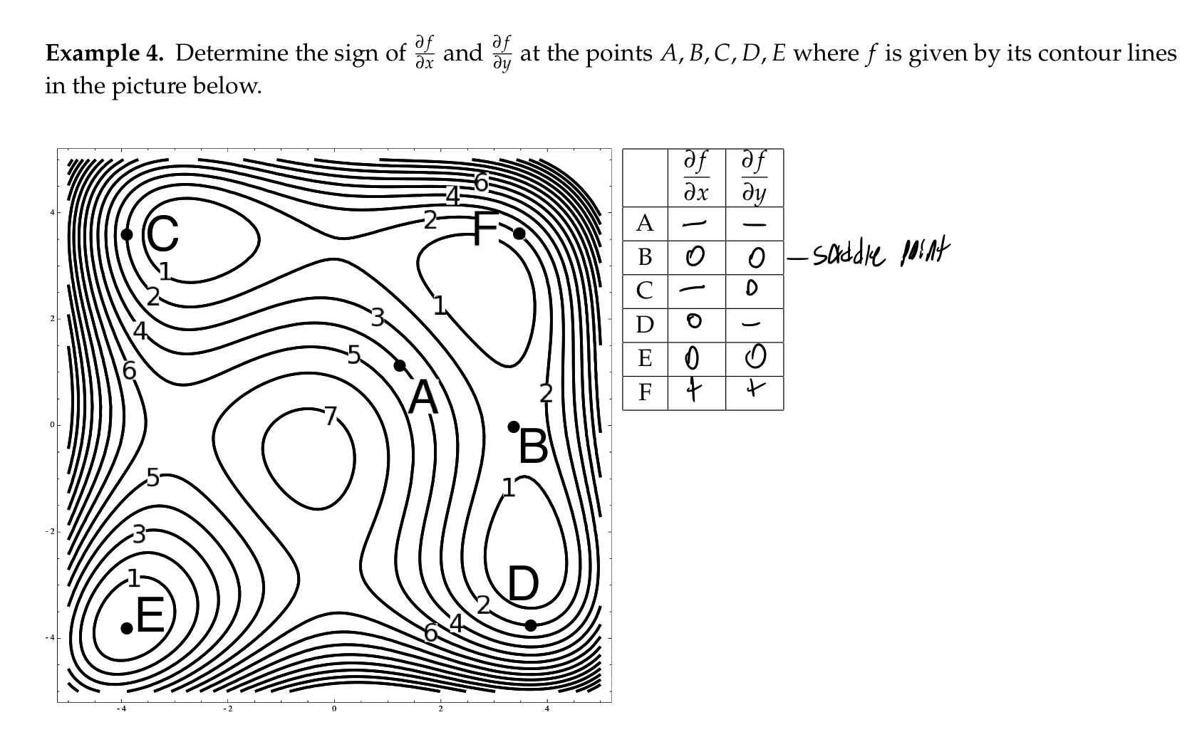
Example 11.3.5: Let us find the minimum of $f(x,y)=x^2-3xy+3y^2+5y+2x$.

First, we find the gradientL: $(\nabla f)(x,y)=\begin{bmatrix} 2x - 3y + 2 \\ -3x + 6y + 5 \end{bmatrix}$

We can now pick an arbitrary point on $f$ for $a$, take $(0,0)$. Then we will move in the direction of the negative gradient: $a+t(\nabla f)(a)$ for some $t<0$ with small absolute value. Basically, we move in the direction of the negative gradient with magnitude $|t|$ and the length $||(\nabla f)(a)||$ to tell us how far we have moved.

Now we pick some arbitrary $t$, say $t=-0.1$.

Finally, we evaluate the above expression, keeping t constant and adjusting $a$–just sequentially adding the vector which indicates the direction of maximum decrease until that vector is 0, or close to it.

Notice we are gradually approaching some value, if we repeat this a hundred or a thousand times, we will have a very accurate approximation of $b \approx (-8.99, -5.33)$. To verify this we can solve the system of equations created by our partial derivatives–in this case we find that the minimum is at $(-9, 5\frac{1}{3})$. We can verify it is the minimum, and not just a critical point by using the multivariable second derivative test.

Chapter 12

Constrained optimization via Lagrange multipliers

We now discuss how to maximize or minimize a multivariable function subject to a constraint. We have discussed finding maximums and minimums by looking at where the partial derivatives of functions are negative, and we have also found extrema through traveling incrementally in the direction of the gradient(gradient descent), but now we discuss how to optimize subject to a constraint using gradients and an auxiliary constant: $\lambda$

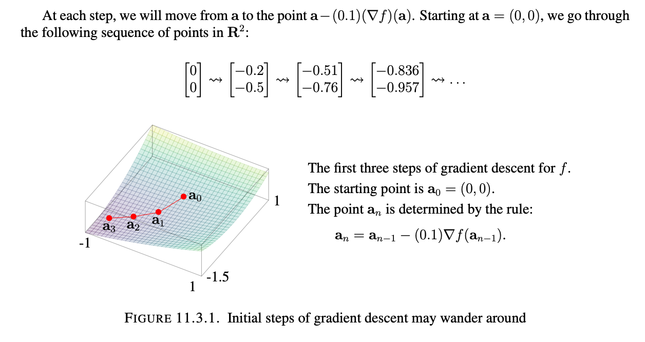
Consider the unit sphere $S$ centered at the origin in $\mathbf{R}^3$, and $f(x,y,z)=z$. The sphere $S$ is defined by $x^2+y^2+z^2=1$, so for $g(x,y,x)=x^2+y^2+z^2$ finding the extrema for $z$ on the sphere $s$ is the same as finding the points in the region $g=1$ at which $f$ attains maximal or minimal values.

By staring at the sphere $S$, we see by inspection that $f$ attains its maximal value on $S$ at the north pole $p=(0,0,1)$ and attains its minimal value at $-p$. These two points are not local extrema for $f$, rather that subject to the constraining sphere, they are the maximal/minimal values that $f$ attains. For tiny $t>0$, at the points (0,0,1+t) close to $p$ the value of $f$ there is bigger than the maximal value $f(p)$, and similar logic follows for $(0,0,-1-t)$. *Basically the “maximum” subject to the constraint is hardly ever a maximum of $f$ globally/locally so there is no need for $\nabla f$ to vanish there.

There is something interesting, however, about the gradient of $f$ at the points where $f$ attains an extreme value on $S$.

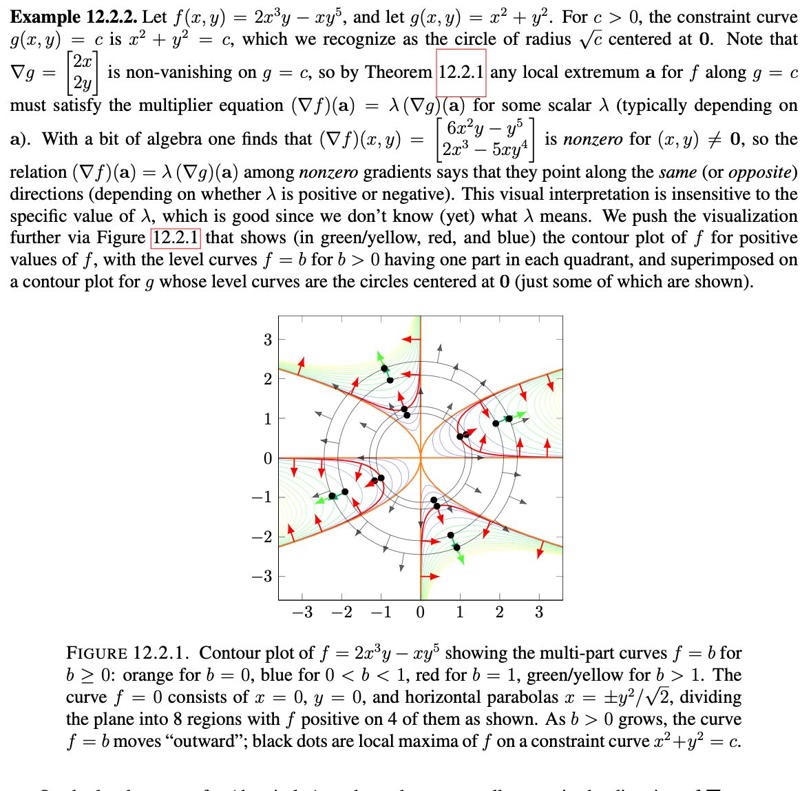
If we look at the gradient of $g$ included below and compare that with the gradient of $f$, then we find that the only points for which these vectors (remember gradients produce a vector output) coincide are the maximal/minimal values of $f$ subject to the constraint function $g$. Essentially the gradient of $f$ is some scalar multiple of the gradient of $g$.

The reason why these vectors coincide only at the extreme values of $f$ subject to the constraint has to do with the level curves of both, and the properties of the gradient related to level curves.

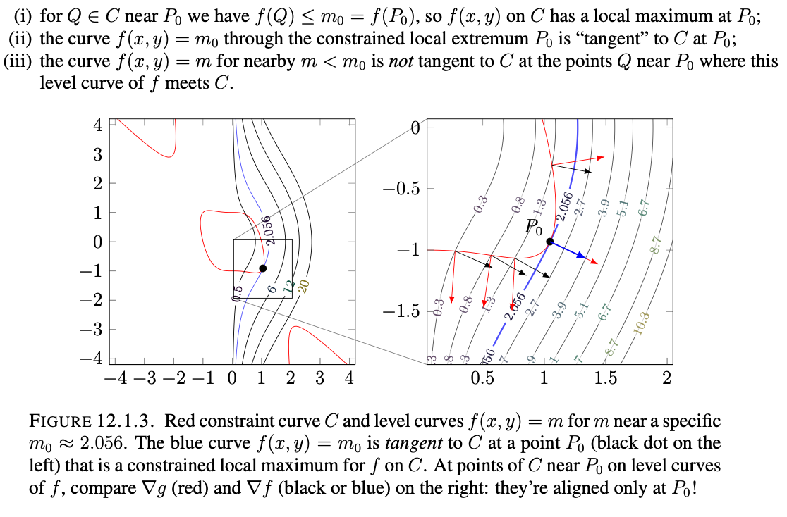
We can reinterpret the level curves’ tangency as the two functions having the same gradient at $P_0$, since the gradient at that point will always be normal to the tangent line of the level curve.

If we imagine all the level curves of $f$, and we plot out the $g(x,y)=c$ it makes sense that the only points where $f$ is going to be maximized subject to the constraint is going to be where the curves coincide with $g$. At these points, when the gradients coincide, it is impossible to increase/decrease $f$ further without violating the constraint.

Theorem 12.2.1: Suppose $f$: $\mathbf{R}^n$->$R$ and $g$: $\mathbf{R}^n$->$R$ are functions, and consider the problem of finding a local maximum(or local minimum) of $f$ on the region where $g(x)=c$. If a local extrema for $f$ on the constraint region occurs at $a$ then either $(\nabla g)(a)=0$ or $(\nabla f)(a)=\lambda(\nabla g)(a)$ for some scalar $\lambda$ that may depend on $a$.

We do not know $\lambda$; but we can solve for it using the system of equations that we obtain above.

It can be the case that there are no constrained global extrema. If $f=xy$ and we restrict it with some equation $y=x^2-3$ then we have $f(x,x^2-3)=x^3-x$–which has no global minimum. For actual application questions in physics and economics, etc. we have non-mathematical reasons to know where there is a maximum or minimum on the constraint region.

When $(\nabla g)(a)=0$ we must check the point $a$ and make sure that satisfies the constraint equation, but if it does then it is a perfectly valid point as an extrema of $f$.

General Strategy: To start find the extrema of $f$ subject to a constraint, the following sequence of steps will generally lead to the answer.

(i) Find what the functions $g$ and $f$ are and find their gradients.

(ii) Manipulate the system of equations obtained by setting the gradients equal to each other, by either a) solving for lambda, or b), canceling lambda and writing the variables in terms of eachother.

(iii) Plug this new equality into the constraint equation to find specific numerical values for the variables. Check each possible variable equality and value!

(iv) Check the values of these points and compare.

(v) Be careful about accidentally canceling variables that can give you more solutions. Also beware of situations in which there is no global max/min.

Chapter 13

Linear functions, matrices, and the derivative matrix

Here we will discuss what matrices are, what they represent, and what linear functions are. In subsequent sections I’ll go over what linear transformations are, how matrices are relevant to them, and many other applications of matrices.

We know how to express the notion of the derivative of some scalar valued function as $\nabla f$, and we can extend that to a vector-valued function as $\nabla f_i$ for each $f_i$ component function. In this section I’ll describe how to nicely package this into a form that is easily readable and intuitive.

Recall that for a vector valued function $f$: $\mathbf{R}^n$->$\mathbf{R}^m$, and $x \in \mathbf{R}^n$ there is the form $$f(x)=\begin{bmatrix} f_1(x) \\ f_2(x) \\ \vdots \\ f_n(x) \end{bmatrix}$$

To approximate the value of a vector valued function such as $f$ at $x$ near $a$ we would need to, for each $i$, find: $f_i(a)+((\nabla f_i)(a))\cdot{(x_1-a_1, x_2-a_2, …, x_n-a_n)}$. If we consider $n=3$ and $f(x,y,z)$ this already gets very complicated: $$\begin{bmatrix} f_1(x,y,z) \\ f_1(x,y,z) \\ f_1(x,y,z) \end{bmatrix} \approx f(a,b,c) + \begin{bmatrix} \frac{\partial f_1}{\partial x}(a,b,c)(x-a) + \frac{\partial f_1}{\partial y}(a,b,c)(y-b) + \frac{\partial f_1}{\partial z}(a,b,c)(z-c) \\ \frac{\partial f_2}{\partial x}(a,b,c)(x-a) + \frac{\partial f_2}{\partial y}(a,b,c)(y-b) + \frac{\partial f_2}{\partial z}(a,b,c)(z-c) \\ \frac{\partial f_3}{\partial x}(a,b,c)(x-a) + \frac{\partial f_3}{\partial y}(a,b,c)(y-b) + \frac{\partial f_3}{\partial z}(a,b,c)(z-c) \end{bmatrix}$$

We will discuss a shortform of writing this later, but for now we will discuss some classes of scalar valued functions that will become important later.

Definition 13.2.1: A scalar valued function $f$: $\mathbf{R}^n$->$R$ is called

-affine if it has the form $f(x_1,…,x_n)=a_1x_1+a_2x_2+…+a_nx_n+b$ for some numbers $a_1,…,a_n,b$ (s0 $b=f(0)$).

-Linear if it has the form $f(x_1,…,x_n)=a_1x_1+a_2x_2+…+a_nx_n$ for some numbers $a_1,…,a_n$; i.e. it is affine with $b=0$, or equivalently with $f(0)=0$.

A vector valued function $f$: $\mathbf{R}^n$->$\mathbf{R}^m$ (so $f(x)=(f_1(x),…,f_m(x))$) is called::

-affine if each of its component functions $f_i$ : $\mathbf{R}^n$->$R$ is affine.

-linear if each of its component functions $f_i$ : $\mathbf{R}^n$->$R$ is linear.

i.e. linear: $$f(\begin{bmatrix} x \\ y \\ z \end{bmatrix})=\begin{bmatrix} ax + by + cz \\ dx + ey + fz \\ gx + hy + iz \end{bmatrix}$$

Definition 13.3.1: An $m x n$ matrix is a rectangular array $A$ of numbers presented like this: $$\begin{bmatrix} a_{1,1} & a_{1,2} & \cdots & a_{1,n} \\ a_{2,1} & a_{2,2} & \cdots & a_{2,n} \\ \vdots & \vdots & \ddots & \vdots \\ a_{m,1} & a_{m,2} & \cdots & a_{m,n} \end{bmatrix} $$

The collection of entries $[a_{i,1}, a_{i,2}, \cdots a_{i,n}]$ along the $i$th layer horizontal (with $i=1$ along the top side) is called the $i$th row, and the collection of entries $\begin{bmatrix} a_{1,j} \\ a_{2,j} \\ \vdots \\ a_{m,j} \end{bmatrix}$ along the $j$th vertical layer (with $j=1$ along the left side) is called the $j$th column.

The entry at the $i$th row and $j$th column is denoted the $ij$ entry.

For a linear vector valued function, we denote the matrix-vector product(inputting a vector into our vector valued function) as such:

Definition 13.3.4: If $A$ is an $m x n$ matrix, and $x \in \mathbf{R}^n$, the matrix-vector product $Ax \in \mathbf{R}^n$ is defined as: $$\begin{bmatrix} a_{1,1} & a_{1,2} & \cdots & a_{1,n} \\ a_{2,1} & a_{2,2} & \cdots & a_{2,n} \\ \vdots & \vdots & \ddots & \vdots \\ a_{m,1} & a_{m,2} & \cdots & a_{m,n} \end{bmatrix} \begin{bmatrix} x_1 \\ x_2 \\ \vdots \\ x_n \end{bmatrix}=\begin{bmatrix} a_{1,1}x_1 + a_{1,2}x_2 + \cdots + a_{1,n}x_n \\ a_{2,1}x_1 + a_{2,2}x_2 + \cdots + a_{2,n}x_n \\ \vdots \\ a_{m,1}x_1 + a_{m,2}x_2 + \cdots + a_{m,n}x_n \end{bmatrix}$$

In other words, if we write $r_1, …, r_m$ for the rows of $A$(so these are n-vectors), then $$Ax=\begin{bmatrix} r_1 \cdot{x} \\ r_2 \cdot{x} \\ \vdots \\ r_m \cdot{x} \end{bmatrix} $$

!! If $A$ is an $m x n$ matrix and $x$ is a $d$-vector with $d \neq n$ then the matrix-vector product $Ax$ is not defined!! This makes sense since we need there to be $n$ components of the vector in order to dot it with the $n$ columns of the matrix.

Proposition 13.3.8: A function $f$: $\mathbf{R}^n$->$\mathbf{R}^m$ is linear precisely when $f(x)=Ax$ for an $m x n$ matrix $A$.

This just rephrases the definition of a linear function. In this way, an $m x n$ matrix $A$ is a shorthand way of encoding a linear function from $\mathbf{R}^n$->$\mathbf{R}^m$

Theorem 13.4.1: If $c_1,c_2,…,c_n$ are the columns of $A$ (so viewed as vectors in $\mathbf{R}^m$), which is to say $$A=[c_1, c_2, …, c_n]$$, then $$A\begin{bmatrix} x_1 \\ x_2 \\ \vdots \\ x_n \end{bmatrix}=x_1c_1+x_2c_2+…+x_nc_n \in \mathbf{R}^m$$.

In particular, the matrix vector product is a specific linear combination of the columns of the matrix; the vector tells us which linear combination to take(i.e. it records the coefficients in the linear combination)

As we write down the columns $c_1, c_2, …, c_n$ from left to right, each appears in the linear combination multiplied against a scalar that varies through the entries $x_i$ in the vector part of the matrix-vector product read top-down.

Theorem 13.4.5: For a linear function $f(x) = Ax$, in the matrix $A$ has as its respective columns $f(e_1), f(e_2),…,f(e_n)$ are the “coordinate vectors.” In other words, the matrix vector product $Ae_j$ is the $j$th column of the matrix $A$. In particular, we can reconstruct the matrix $A$ from the function $f(x)=Ax$.

Now we return to the shorthand form of derivatives of vector valued functions.

Definition 13.5.1: Let $f$: $\mathbf{R}^n$->$\mathbf{R}^m$ be a vector valued function $f(x)=\begin{bmatrix} f_1(x) \\ \vdots \\ f_m(x) \end{bmatrix}$ with scalar valued components $f_1,…,f_m$: $\mathbf{R}^n$->$R$. The derivative matrix of $f$ at point $a \in \mathbf{R}^n$ is the $m x n$ matrix: $$(Df)(a)=\begin{bmatrix} \frac{\partial f_1}{\partial x_1} & \frac{\partial f_1}{\partial x_2} & \cdots & \frac{\partial f_1}{\partial x_n} \\ \frac{\partial f_2}{\partial x_1} & \frac{\partial f_2}{\partial x_2} & \cdots & \frac{\partial f_2}{\partial x_n} \\ \vdots & \vdots & \ddots & \vdots \\ \frac{\partial f_m}{\partial x_1} & \frac{\partial f_m}{\partial x_2} & \cdots & \frac{\partial f_m}{\partial x_n} \end{bmatrix}$$ with all partial derivatives $\frac{\partial f_i}{\partial x_j}$ evaluated at the point $a$. (Also called the Jacobian matrix).

For a scalar valued function $f$: $\mathbf{R}^n$->$R$ (m=1), the derivative matrix will be flipped so that each partial derivative is one of the component outputs for the n-vector.

Theorem 13.5.8: The best linear approximation to $f$ : $\mathbf{R}^n$->$\mathbf{R}^m$ at $a \in \mathbf{R}^n$ is given by the $m x n$ derivative matrix $Df(a)$: we have the optimal approximation of m-vectors: $$f(x) \approx f(a) + ((Df(a)))(x-a)$$

Add some examples

Chapter 14

Linear transformations and matrix multiplication

So we know what matrices are, what their product with vectors look like, and some ways we can package some concepts such as the derivative within a matrix; but now we look into what they actually represent and some other ways we can work with them (which will become very important in later chapters).

Matrices encode the information necessary for linear transformations, which are ways of manipulating space in such a way that we maintain properties of linearity. I will elaborate on this in a later definition but for now this is sufficient. While this way of describing what matrices do is certainly correct, I find the way that 3blue1brown puts it to be far more insightful. Just think of the columns of the matrix $A$ as encoding where the basis vectors $(e_1,e_2,…,e_n) \in \mathbf{R}^n$ land in this new transformation of space. Thinking in terms of physics terms, we can interpret it as where the $\hat{i}, \hat{j}, \hat{k}$ vectors land in our new space. In this way we can think of any vector in our original space expressed by some combination of $\hat{i}, \hat{j}, \hat{k}$ in terms of $\hat{i}’, \hat{j}’, \hat{k}’$ where $\hat{i}’, \hat{j}’, \hat{k}’$ are given by the columns of the matrix.

Thinking of it this way, the properties of linearity become quite obvious.

1. the matrix vector product can be extended to scalars, by simply factoring out the scalar from the product and applied to the resulting vector.

2. the matrix vector product can be applied to vectors separately, and since the output vectors are essentially linear combinations of the same vectors(altered basis vectors), any vectors produced by combining these vectors will lie in the same linear subspace.

Definition 14.1.1: A function f : $\mathbf{R}^n$->$\mathbf{R}^m$ is called:

-a linear function, or a linear transformation, if there is an $mxn$ matrix $A$ for which $f(x)=Ax$ for all vectors $x \in \mathbf{R}^n$ (so the $j$th column of $A$ is $Ae_j=f(e_j)$)

-an affine function, or an affine transformation, if there is an $mxn$ matrix $A$ and a vector $b \in \mathbf{R}^m$ for which $f(x) = Ax + b$ for all vectors $x \in \mathbf{R}^n$

Linearity Principle: for $c_1,c_2 \in R$ and $v_1,v_2 \in R^2$ we have $f(c_1v_1 + c_2v_2)=c_1f(v_1) + c_2f(v_2)$.

Tiling Principle: f transforms the tiling of $R^2$ by copies of S into a tiling of $R^2$ by copies of $f(S)$

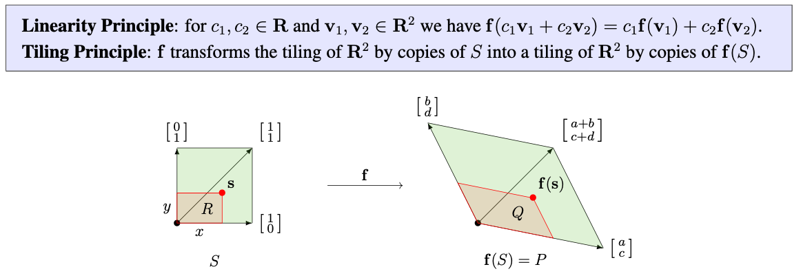
Theorem 14.2.1: A function g : $\mathbf{R}^n$->$\mathbf{R}^m$ is linear precisely when it respects the vector operations: $$g(cx)=cg(x)$$, $$g(x+y) = g(x) + g(y)$$ for all scalars $c \in \mathbf{R}^n$.

If g : $\mathbf{R}^n$->$\mathbf{R}^m$ and h : $\mathbf{R}^p$->$\mathbf{R}^n$ are linear, then so is the composition $g \circ{h}$ : $\mathbf{R}^p$->$\mathbf{R}^m$.

Such operations only work for linear functions, which is part of the reason why linear functions are far more common than their affine counterparts.

Include example 14.2.2

Now we introduce the idea of matrix multiplication. This may sound somewhat daunting, especially for large $m$ and $n$, but if we just think about what we are doing conceptually, it will make perfect sense, and it will even help to explain some of the interesting properties of matrix multiplication.

When we multiply one matrix by another what we are doing is observing an initial linear transformation of $\mathbf{R}^n$ expressed by the $m$-vectors given by the columns of the matrix which represent where each basis vector of $\mathbf{R}^n$ goes. Then we take these transformed basis vectors for some space in $\mathbf{R}^m$, and we treat them as we did the original basis vectors, computing the matrix vector product to see where they land in the newly transformed space.

Formally we have the following:

Definition 14.3.1: Let $A$ be an $mxn$ matrix and $B$ be an $nxp$ matrix as follows: $$\begin{bmatrix} a_{1,1} & a_{1,2} & \cdots & a_{1,n} \\ a_{2,1} & a_{2,2} & \cdots & a_{2,n} \\ \vdots & \vdots & \ddots & \vdots \\ a_{m,1} & a_{m,2} & \cdots & a_{m,n} \end{bmatrix}$$, $$\begin{bmatrix} b_{1,1} & b_{1,2} & \cdots & b_{1,p} \\ b_{2,1} & b_{2,2} & \cdots & b_{2,p} \\ \vdots & \vdots & \ddots & \vdots \\ b_{n,1} & b_{n,2} & \cdots & b_{n,p} \end{bmatrix}$$

Let $T_A$ : $\mathbf{R}^n$->$\mathbf{R}^m$ and $T_B$ : $\mathbf{R}^p$->$\mathbf{R}^n$ be the linear transformations with respective matrices $A$ and $B$ (i.e, $T_a(x)=Ax$ for $x \in \mathbf{R}^n$ , and $T_a(y)=By$ for $y \in \mathbf{R}^p$), so the composition $T_A \circ{T_B}$: $\mathbf{R}^p$->$\mathbf{R}^m$ is a linear transformation. This transformation is denoted $AB$.

Theorem 14.3.2: The entries of $AB$ are the dot products of rows of $A$ with columns of B: if we write $$A=\begin{bmatrix} —-a_1—- \\ —-a_2—- \\ \vdots \\ —-a_m—- \end{bmatrix}$$, $$[b_1, b_2, \cdots, b_p]$$ with rows $a_i \in \mathbf{R}^n$ and columns $b_j \in \mathbf{R}^n$, then we have $$\begin{bmatrix} a_1 \cdot{b_1} & a_1 \cdot{b_2} & \cdots & a_1 \cdot{b_p} \\ a_2 \cdot{b_1} & a_2 \cdot{b_2} & \cdots & a_2 \cdot{b_p} \\ \vdots & \vdots & \ddots & \vdots \\ a_m \cdot{b_1} & a_2 \cdot{b_2} & \cdots & a_m \cdot{b_p} \end{bmatrix}=[Ab_1, Ab_2, \cdots, Ab_p]$$.

$AB \neq BA$

$A(BC)=(AB)C$ This makes sense intuitively when we think about matrices and matrix multiplication as applying successive transformations. Like of course applying one transformation, then another, then another is the same as applying that transformation, then the same consecutive transformations.

Proposition 14.3.7: For $nxn$ diagonal matrices $A$ and $B$, the product matrix $AB$ is also diagonal and is obtained by multiplying the corresponding entries as such $a_{1,1}b_{1,1}, a_{2,2}b_{2,2}, …, a_{n,n}b_{n,n}$: $$\begin{bmatrix} a_{1,1}b_{1,1} & 0 & \cdots & 0 \\ 0 & a_{2,2}b_{2,2} & \cdots & 0 \\ \vdots & \vdots & \ddots & \vdots \\ 0 & 0 & \cdots & a_{n,n}b_{n,n} \end{bmatrix}$$

In particular, $AB=BA$ for these matrices since $a_ib_i=b_ia_i$ for every $i$.

Rotations in $R^2$ and $R^3$: In $R^2$ we have a counterclockwise rotation around the origin by $\theta$ as: $$A_{\theta}=\begin{bmatrix} \cos{\theta} & -\sin{\theta} \\ \sin{\theta} & \cos{\theta} \end{bmatrix}$$

In $R^3$ we have the rotation by an angle $\theta$ counterclockwise around the $y-axis$ as: $$R_y(\theta)=\begin{bmatrix} \cos{\theta} & 0 & \sin{\theta} \\ 0 & 1 & 0 \\ -\sin{\theta} & 0 & \cos{\theta} \end{bmatrix}$$

Other Random Note: Any 3 x 3 matrix whose effect preserves lengths and angles has orthonormal columns.

Chapter 15

Matrix Algebra

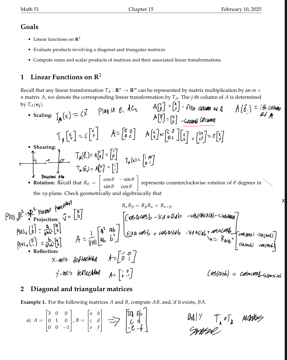
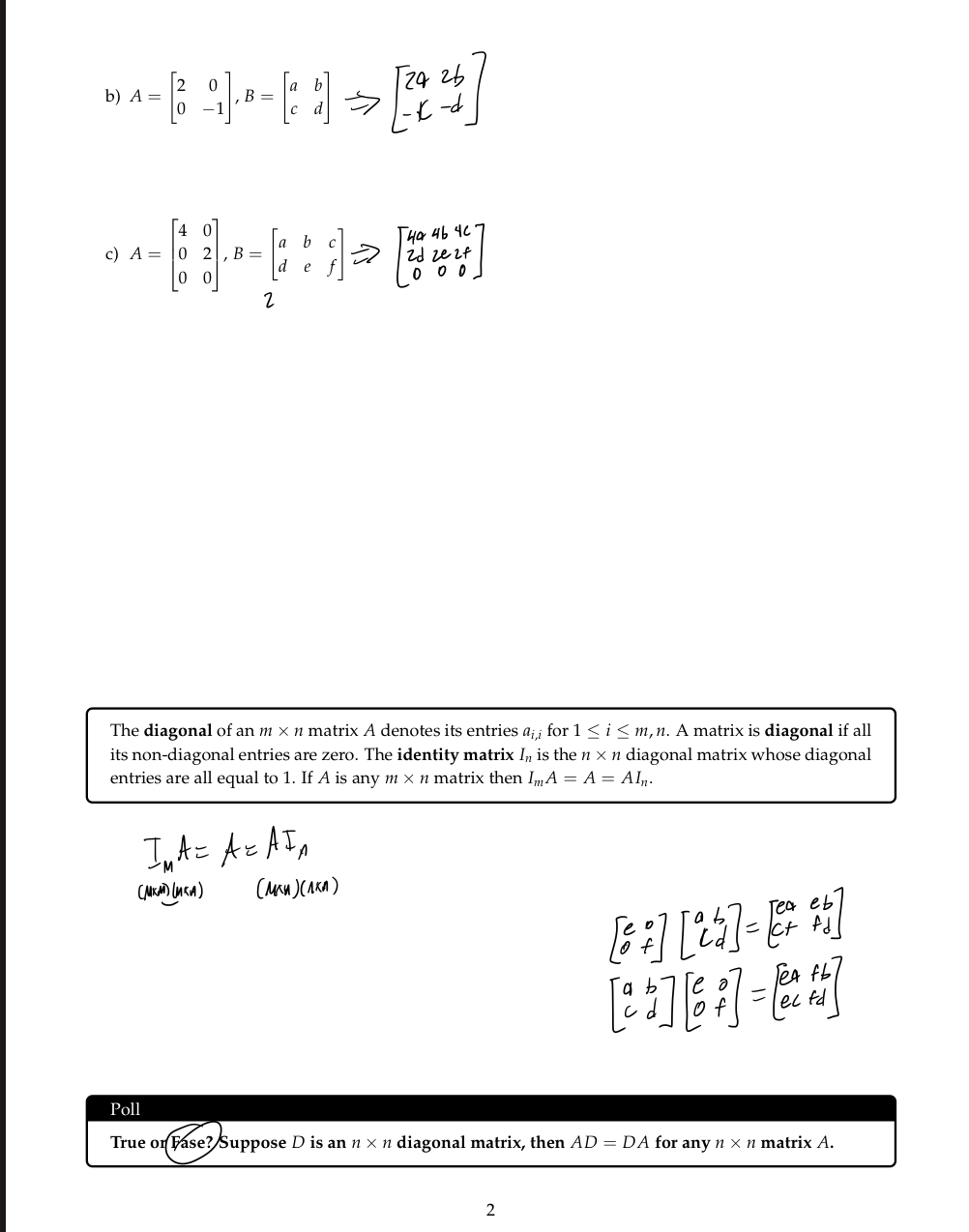
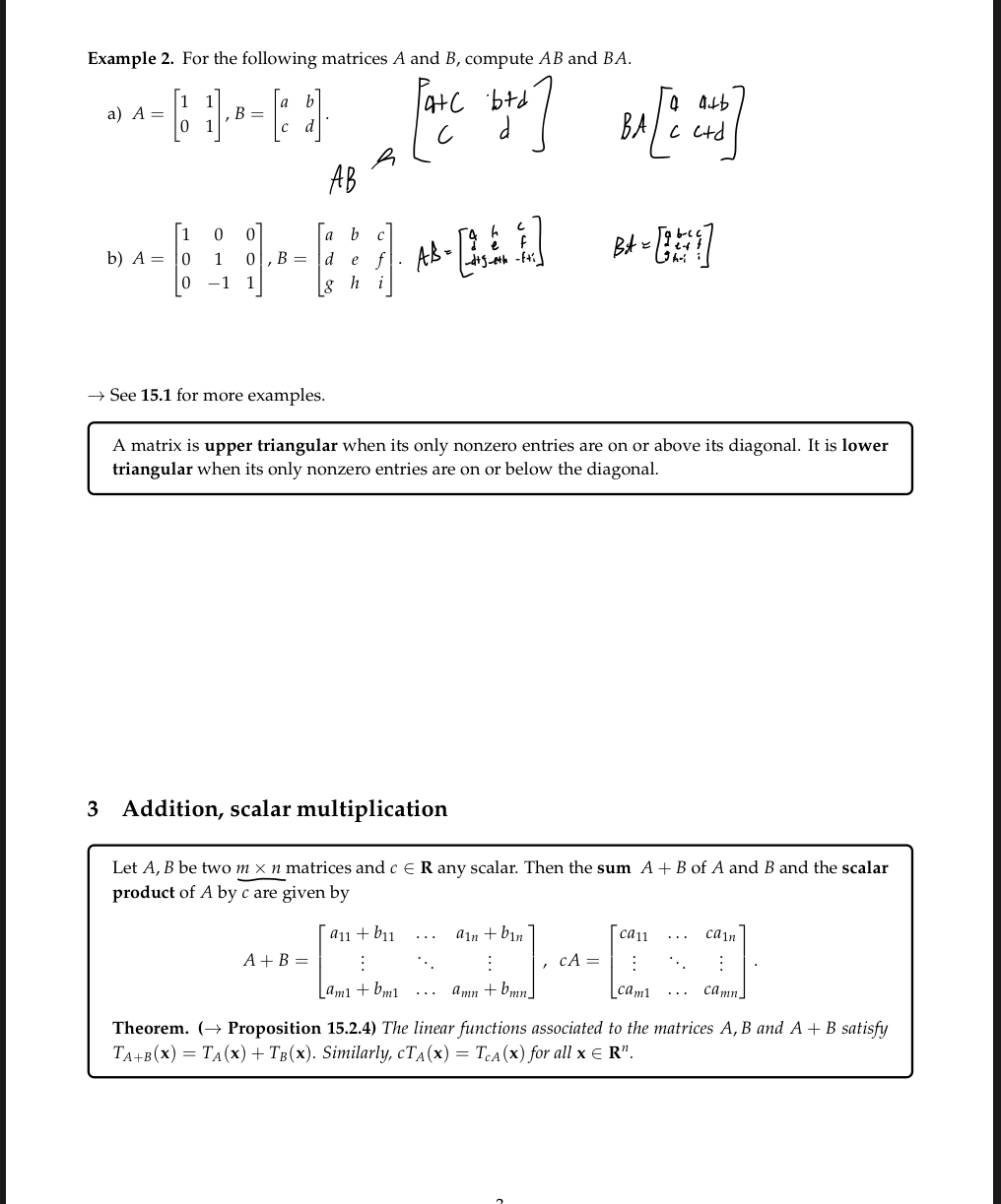
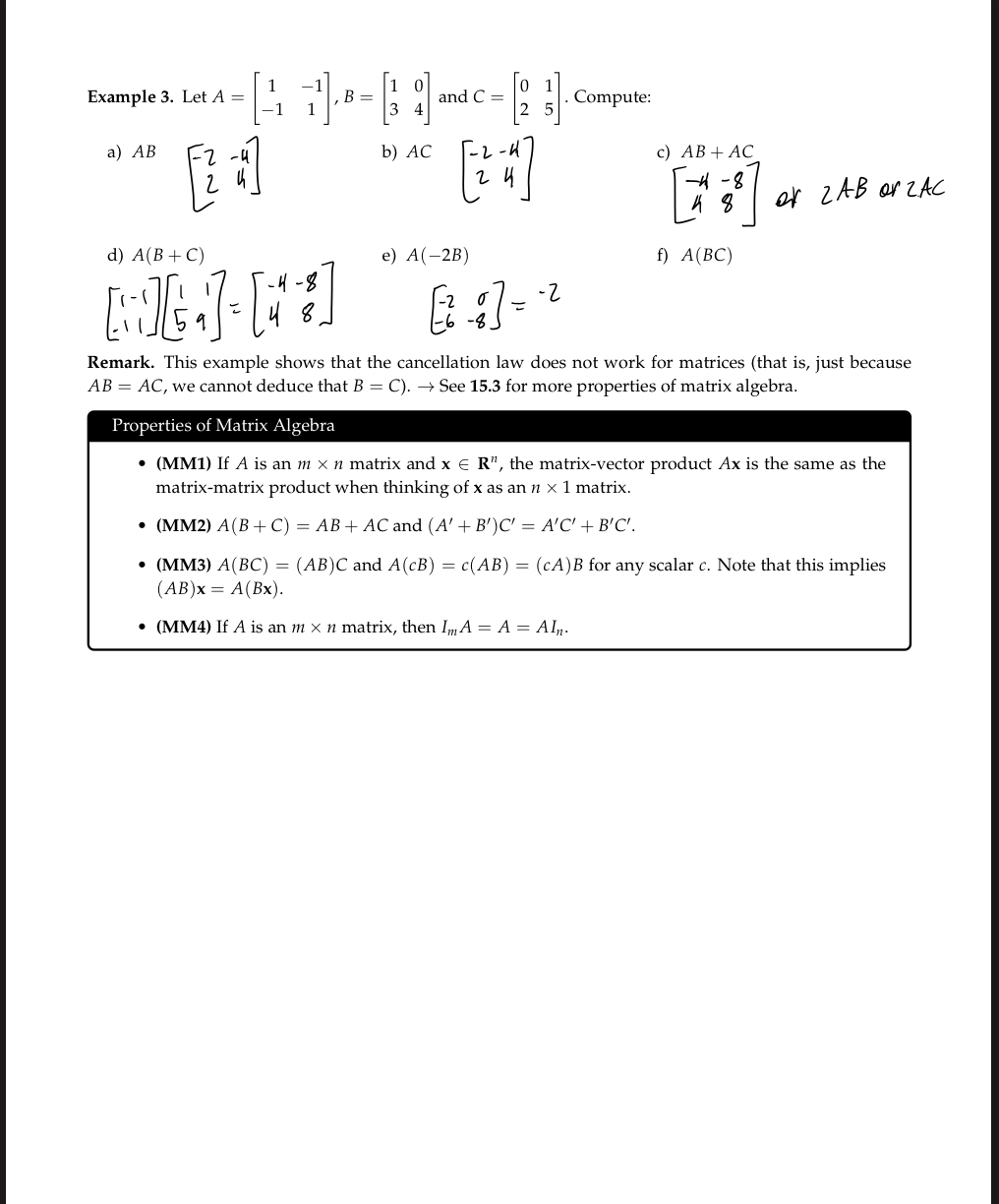
Chapter 16

Markov Matrices

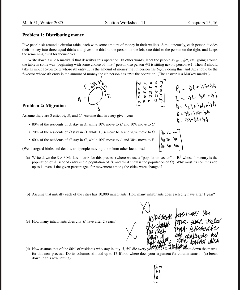
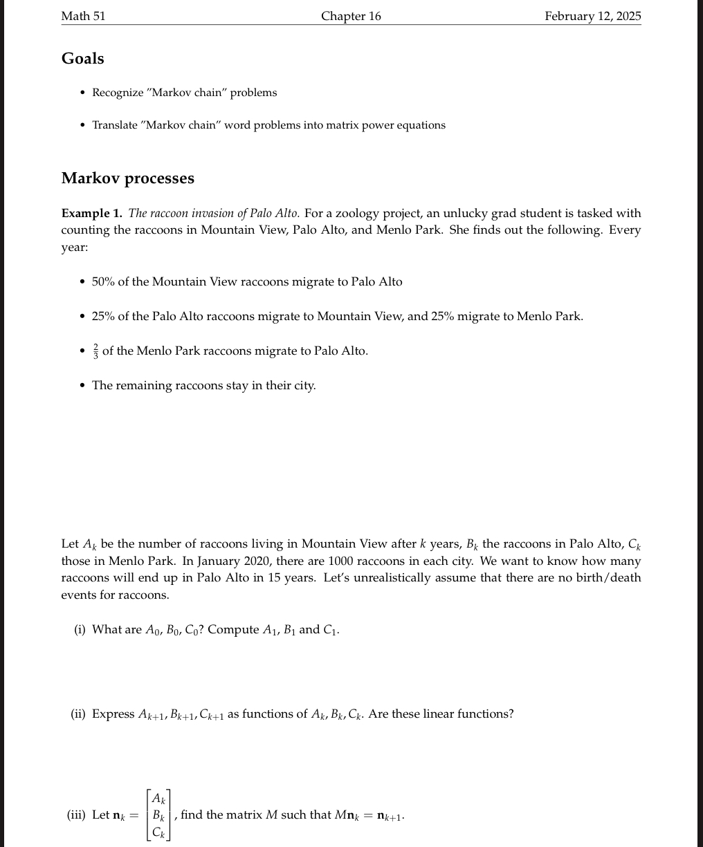
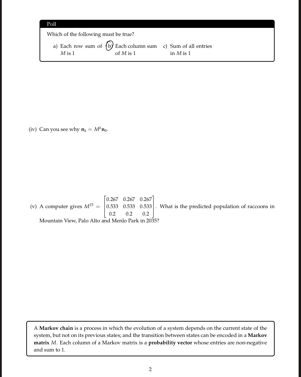
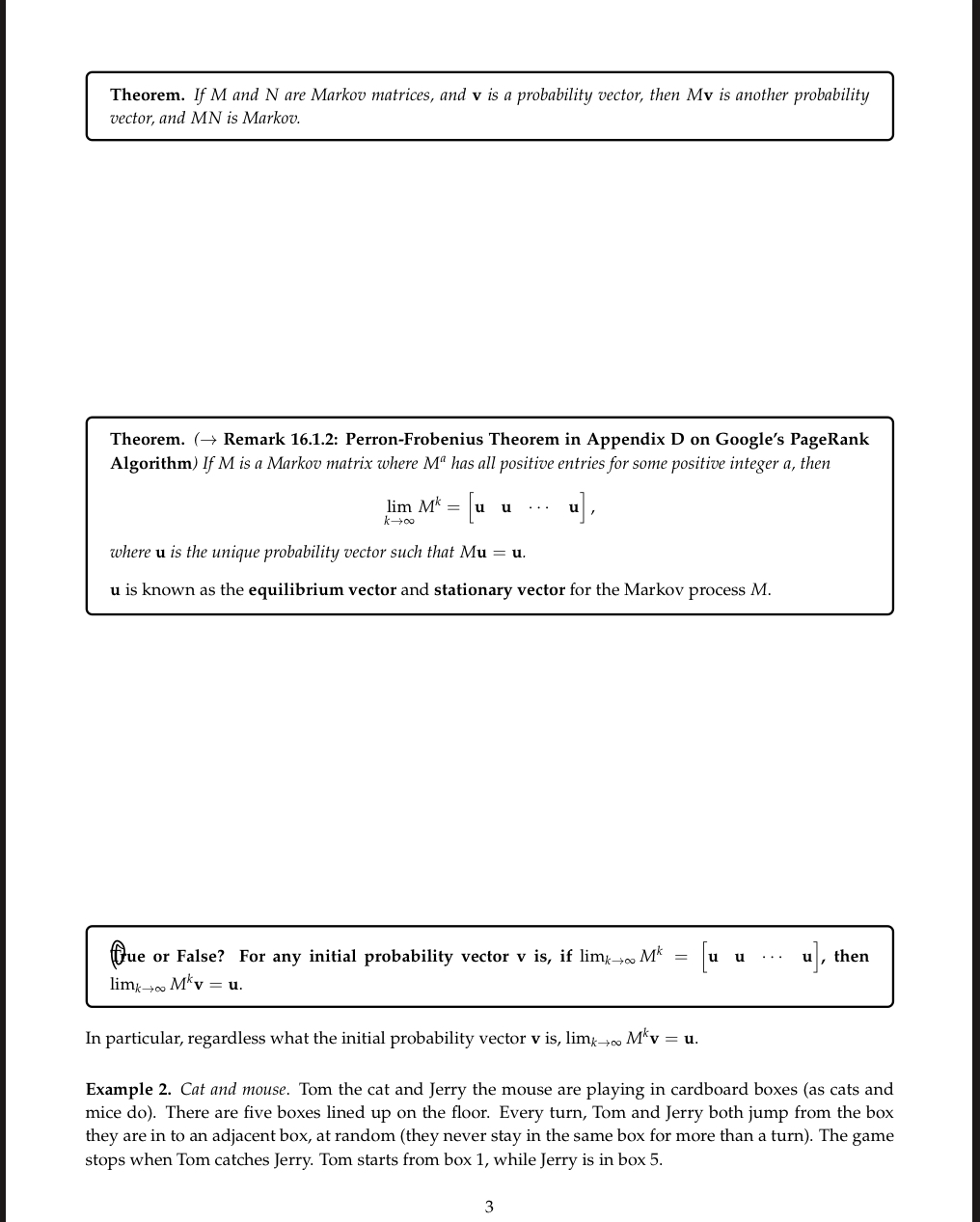
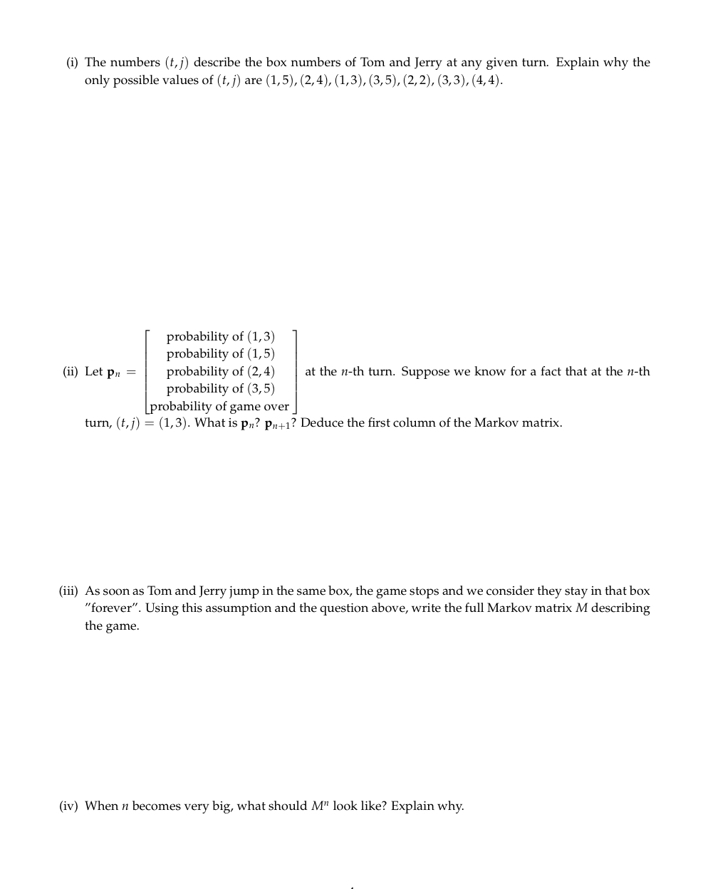
Chapter 17

Matrix Algebra

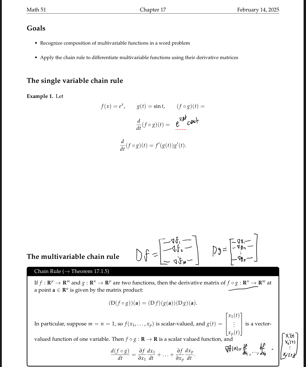
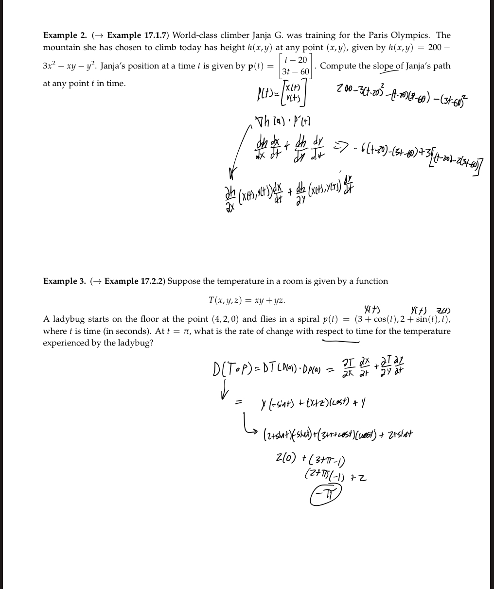
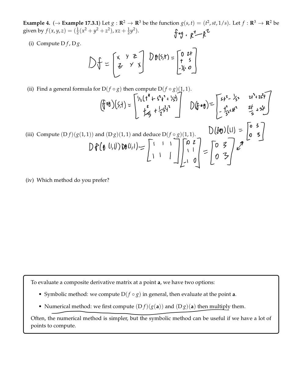
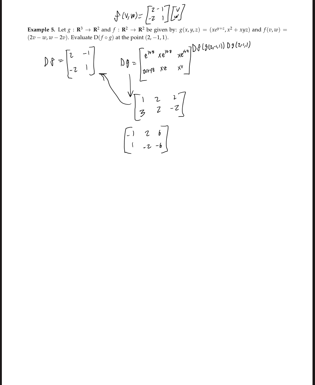
Chapter 18

Matrix Algebra

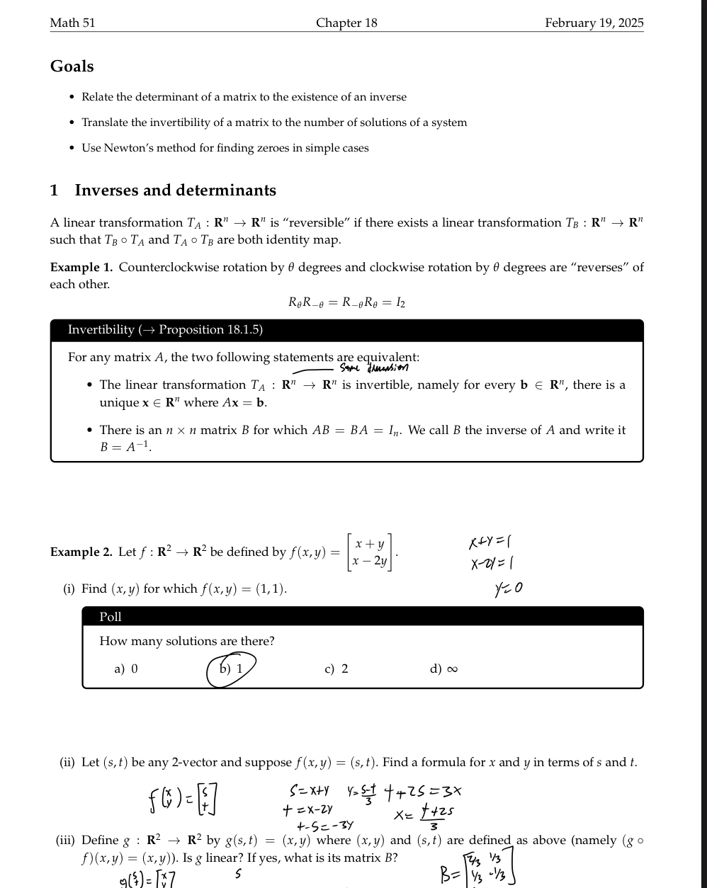
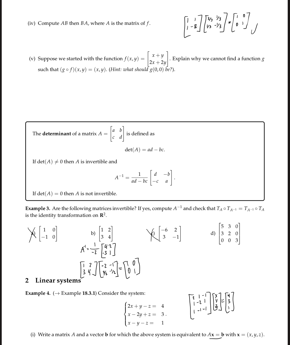
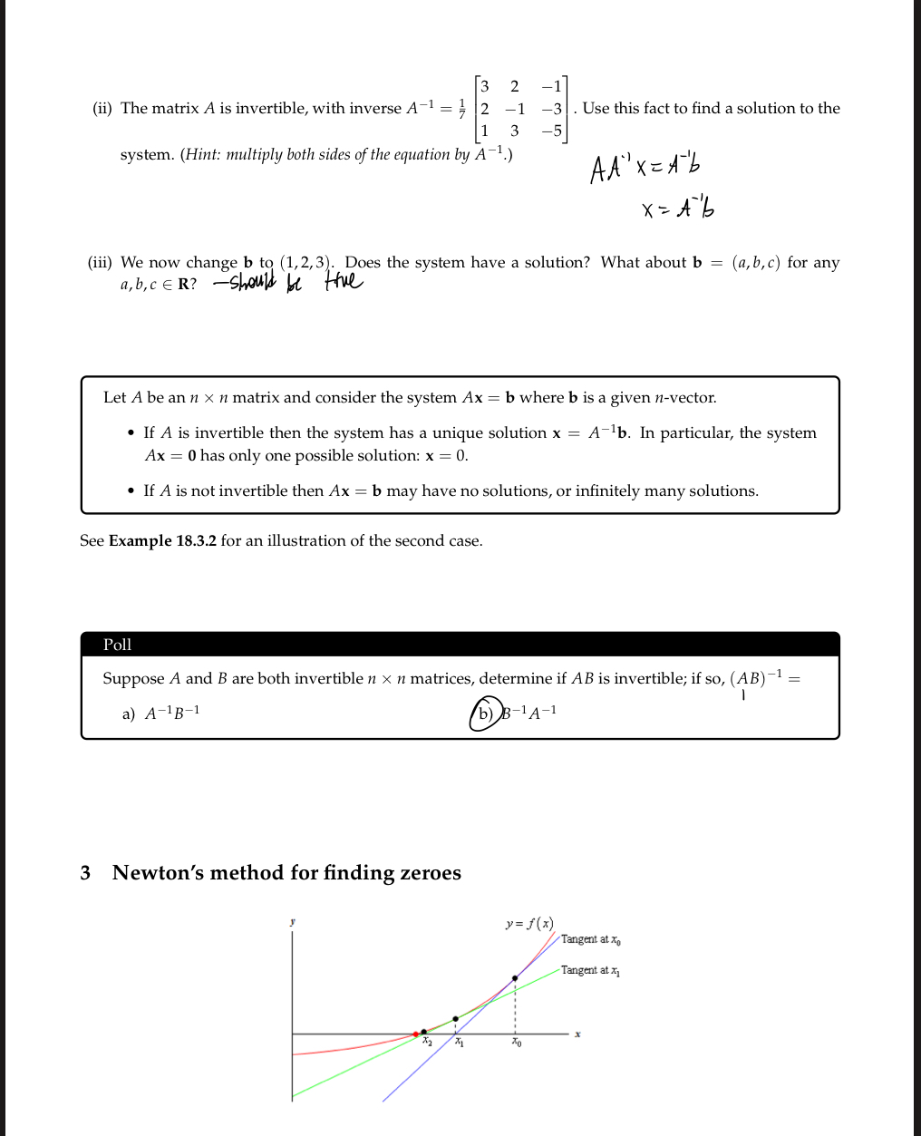
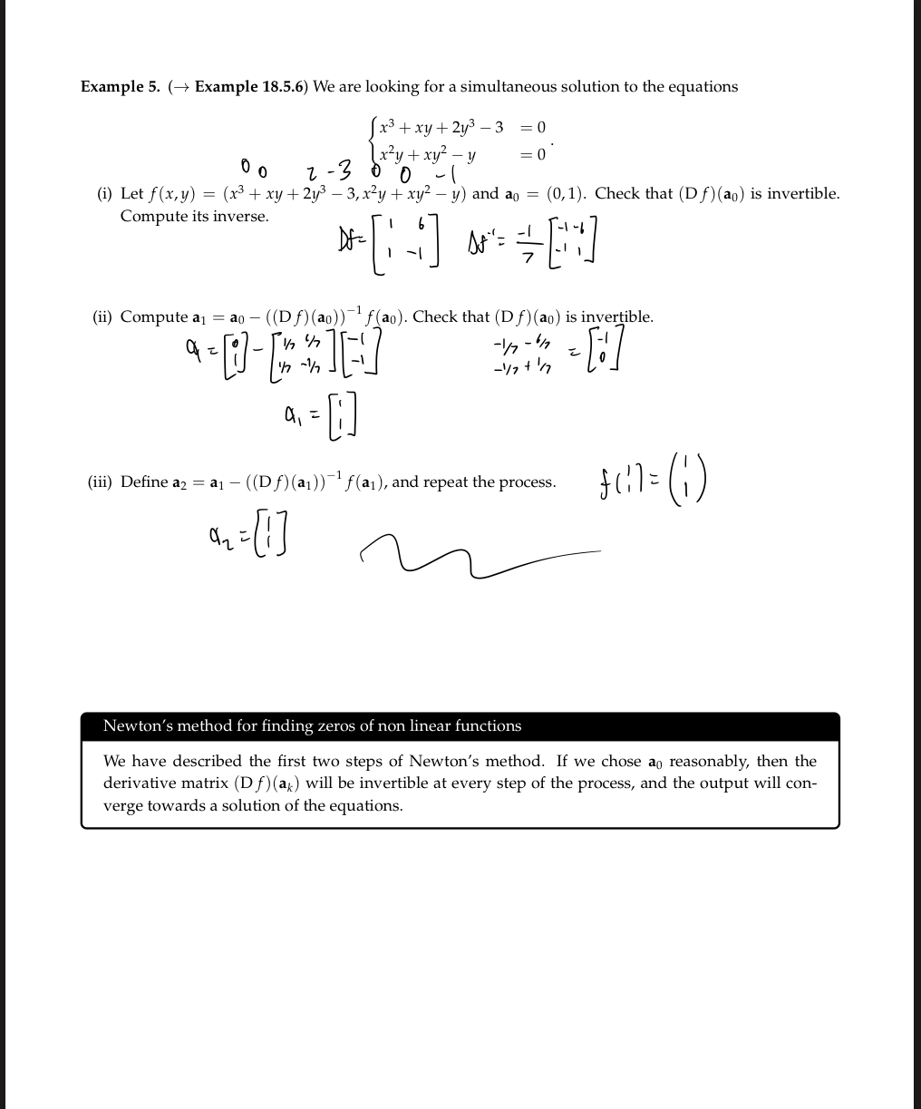
Chapter 19

Matrix Algebra

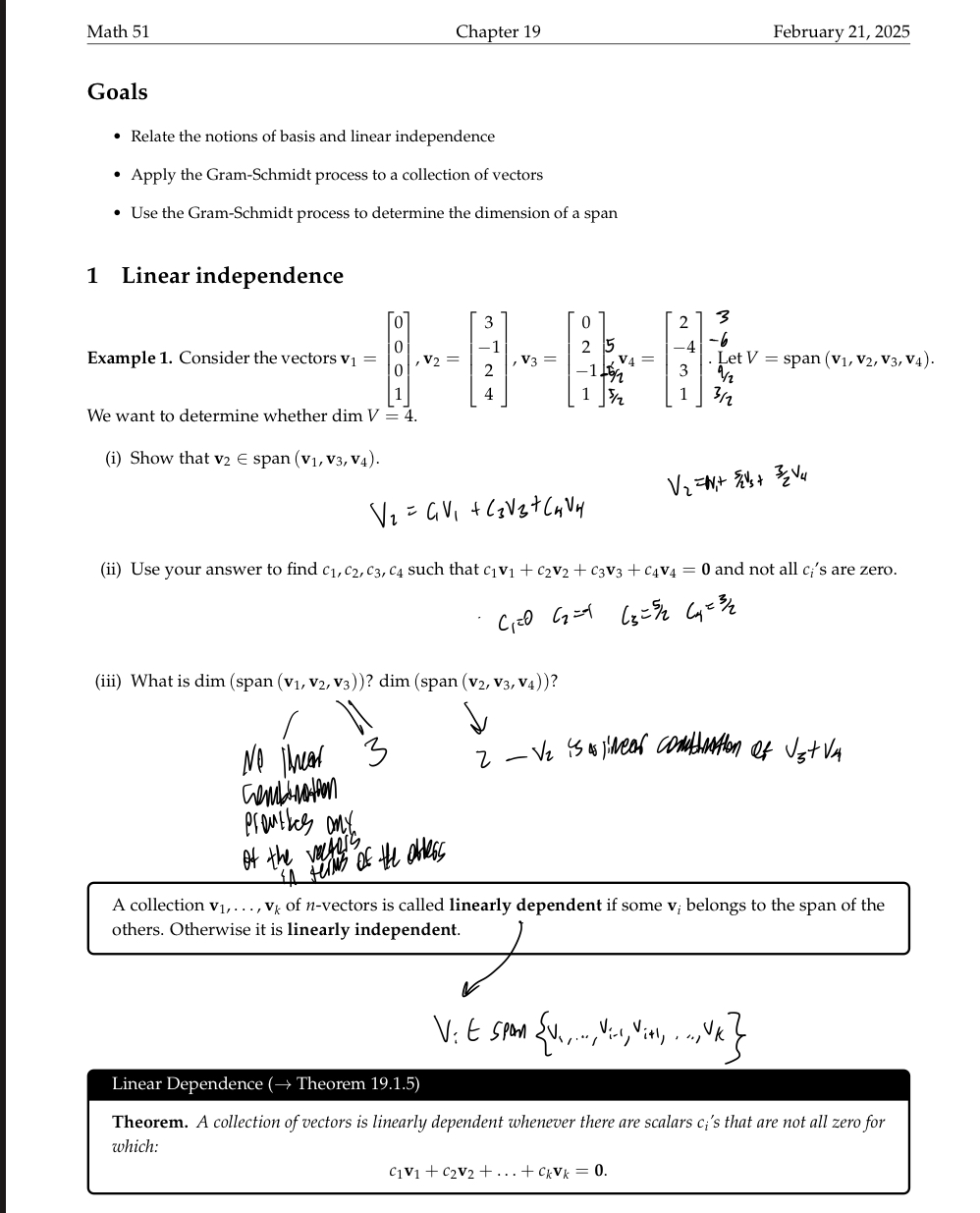
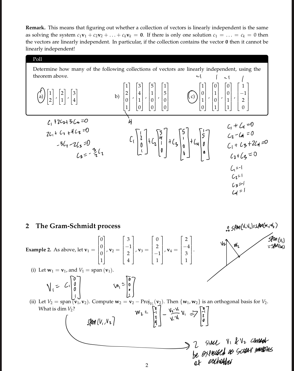
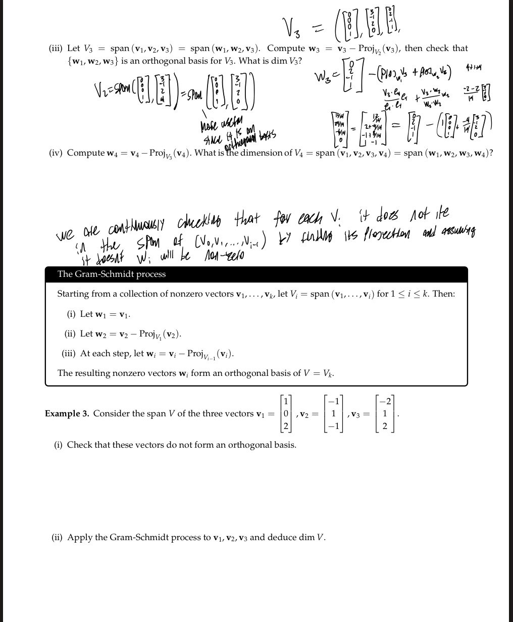
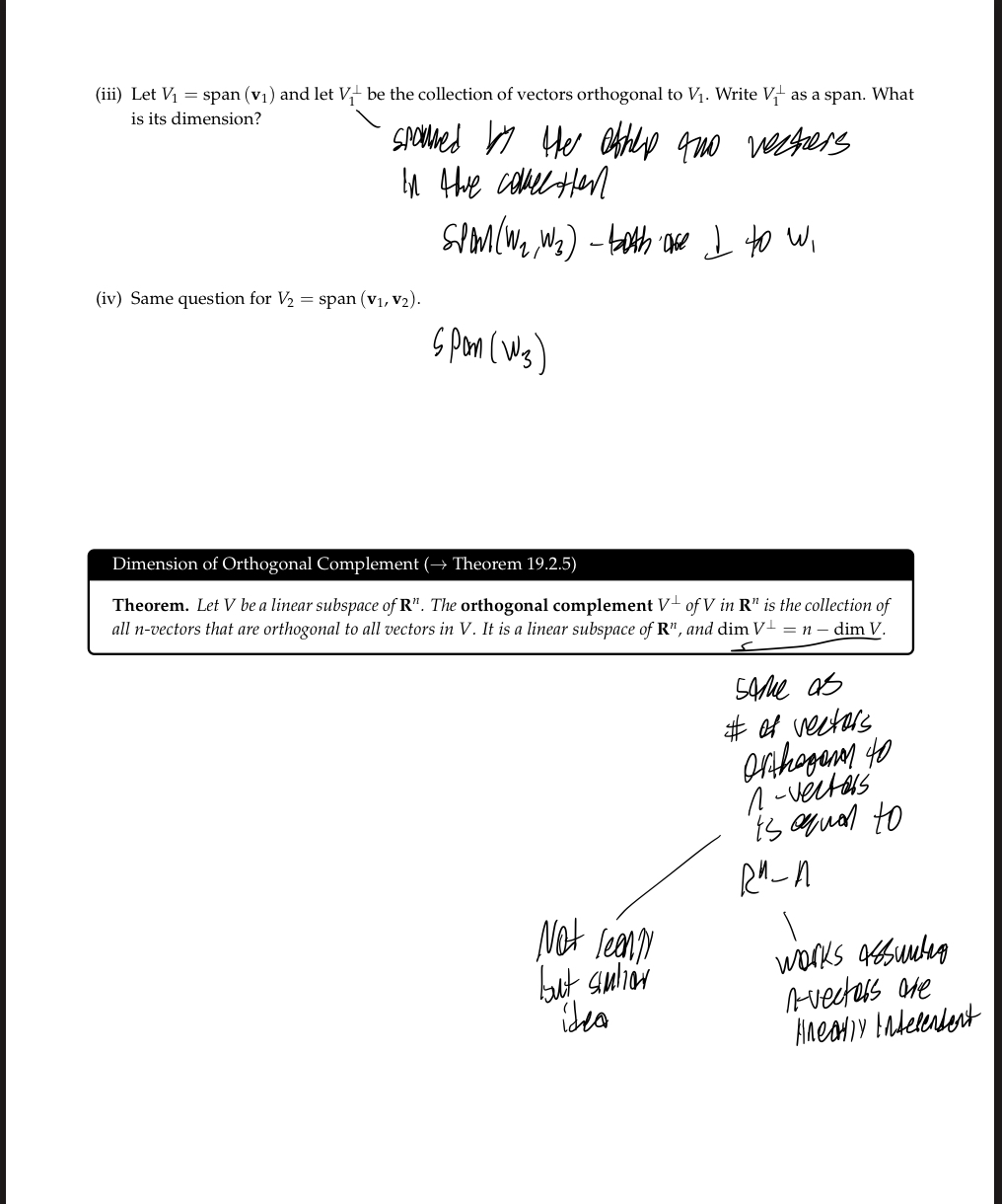
Chapter 20

Matrix Algebra

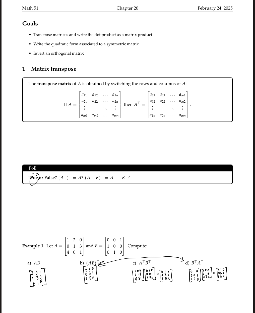
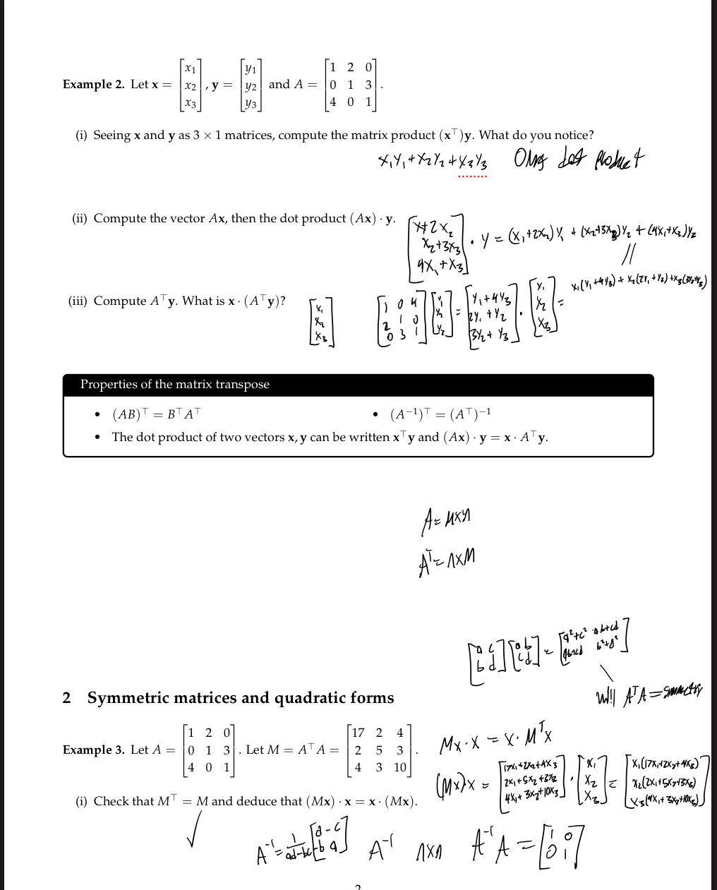
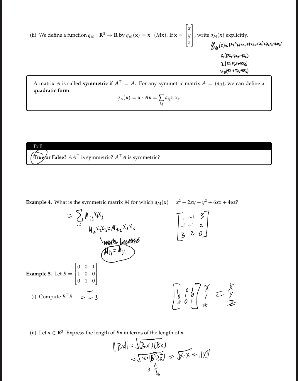
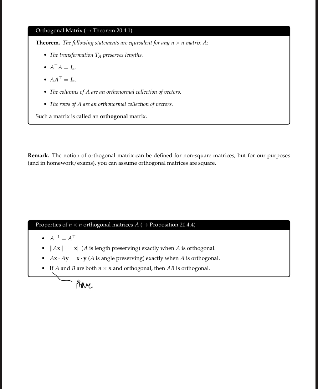
Chapter 21

Matrix Algebra

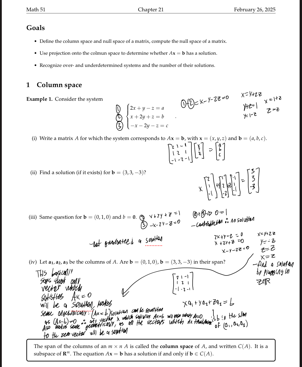
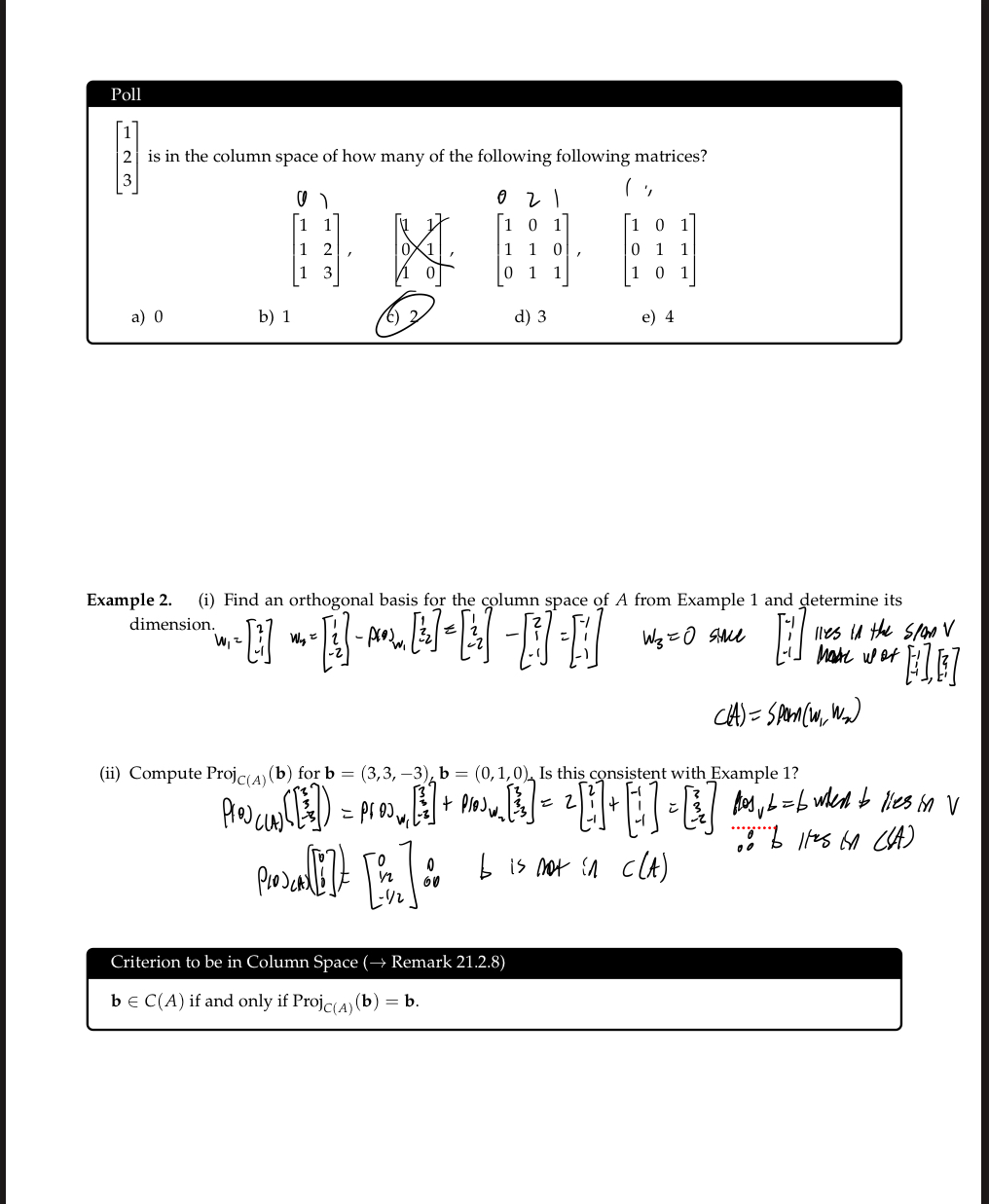
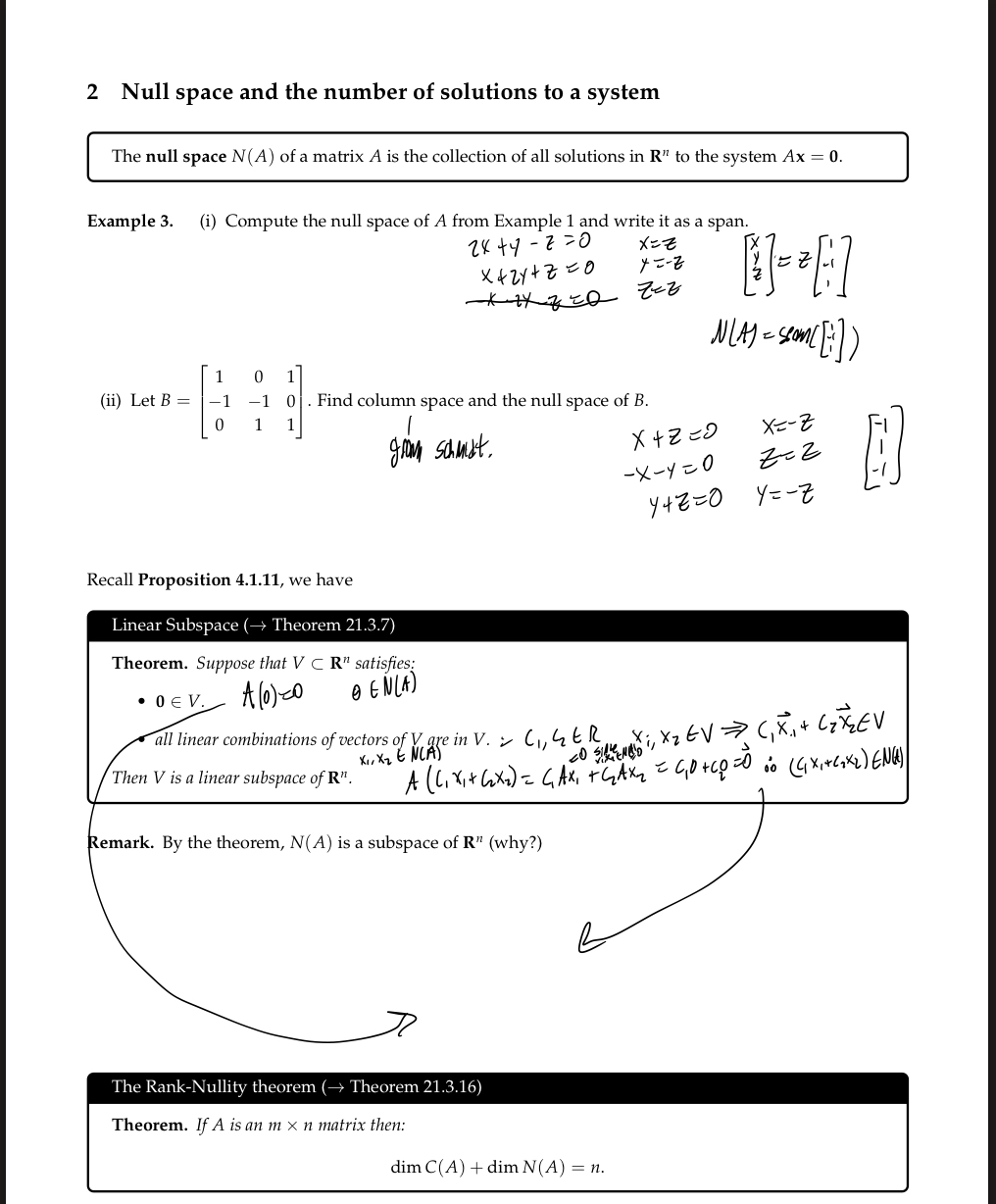
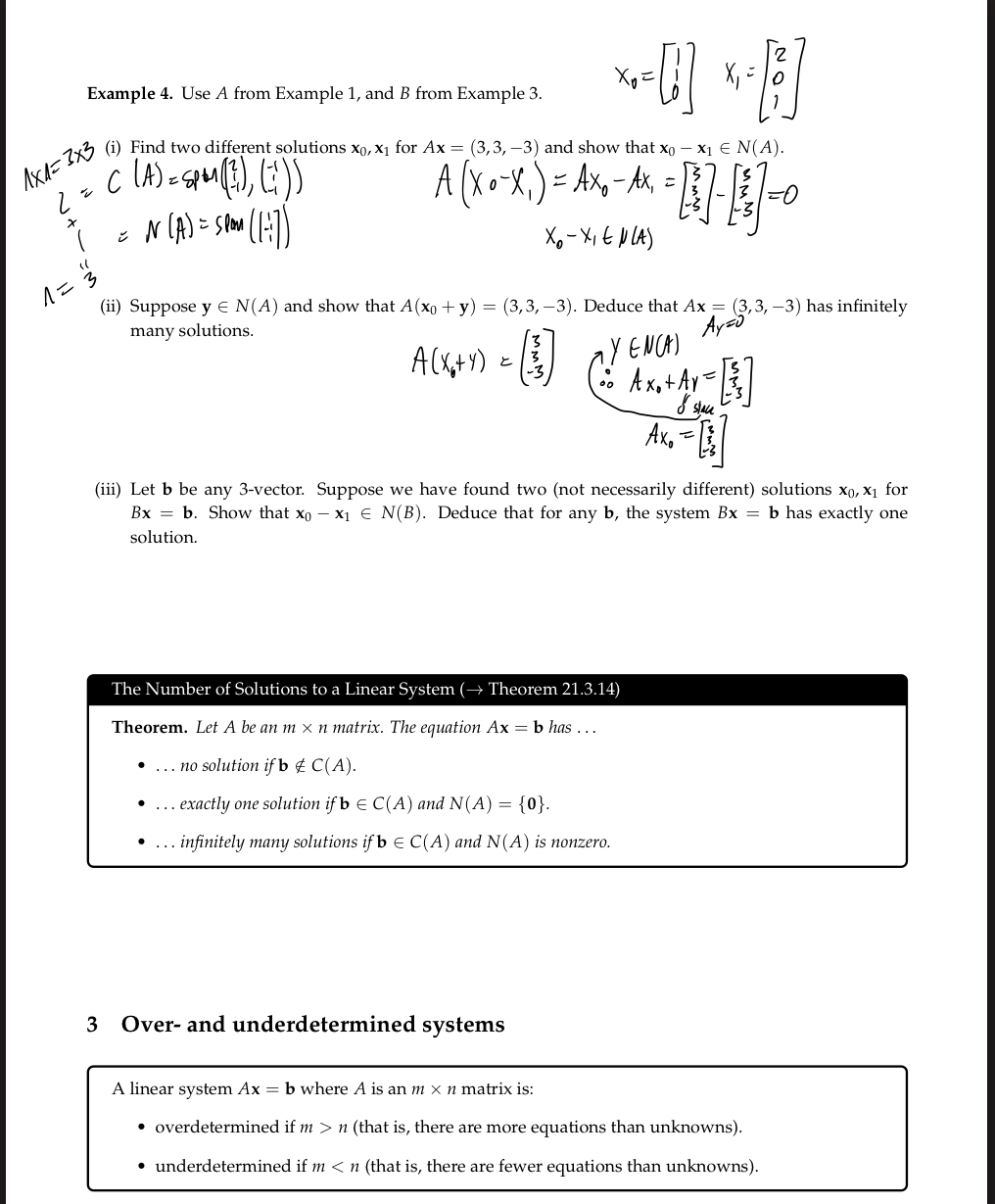
Chapter 22

Matrix Algebra

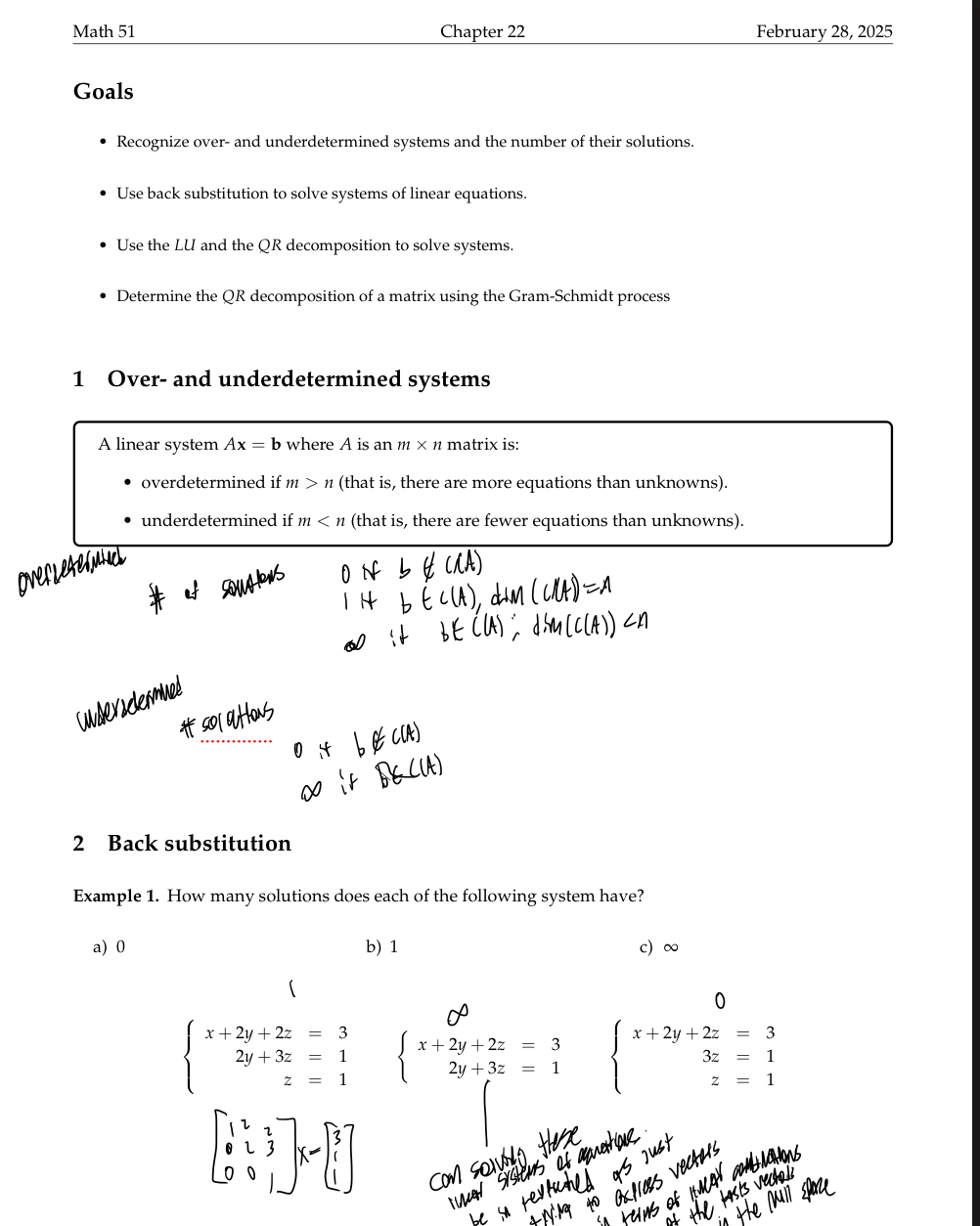
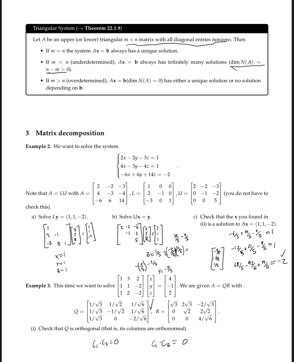
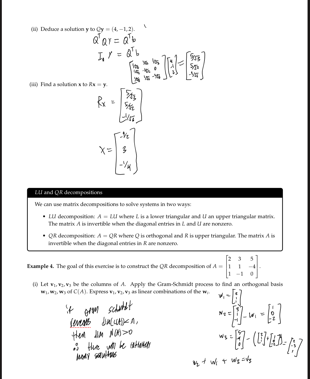
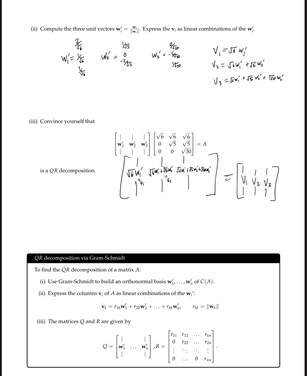
Chapter 23

Matrix Algebra

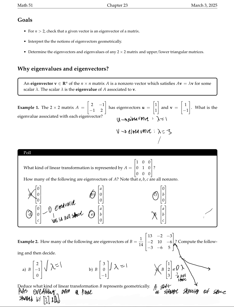
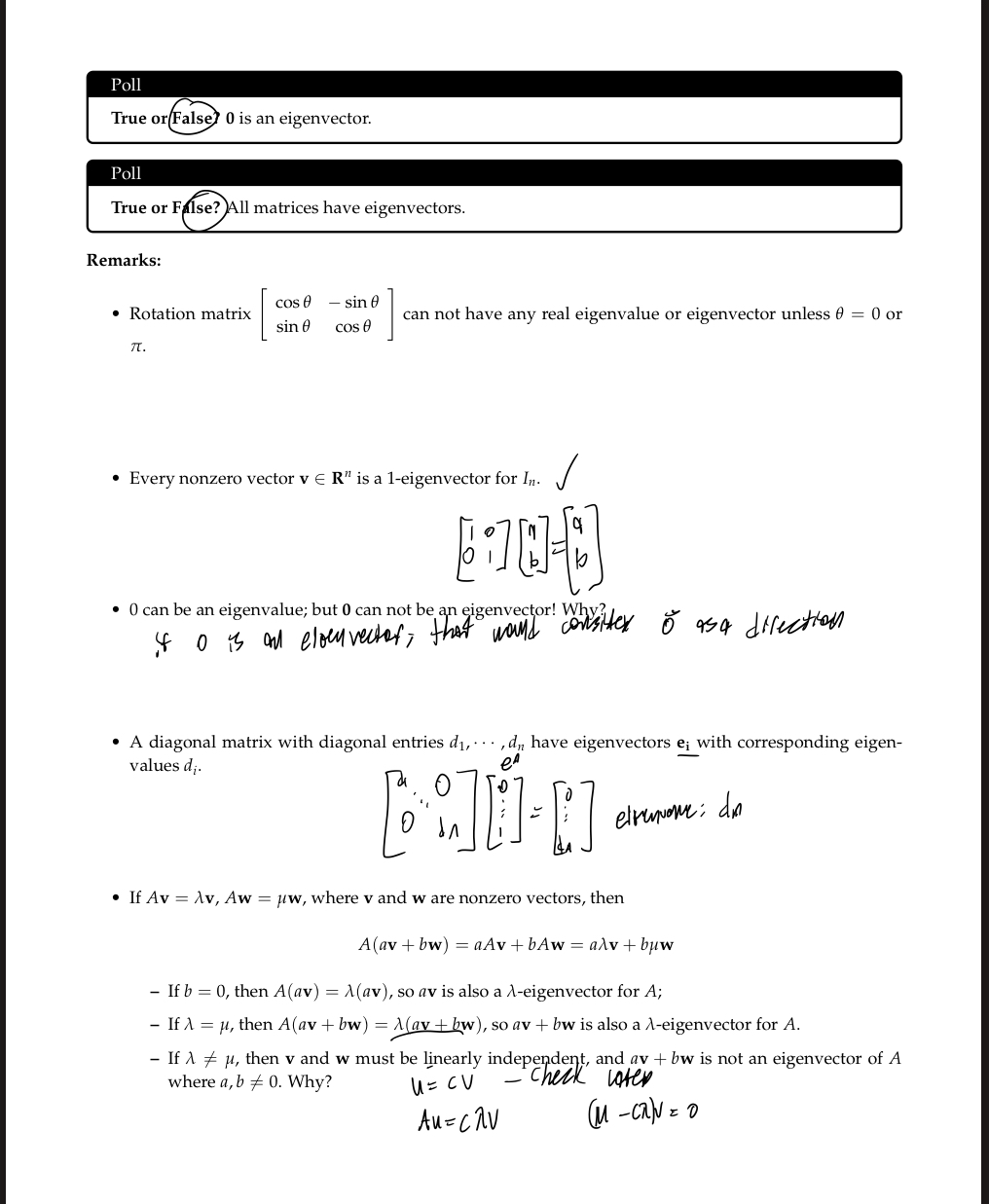
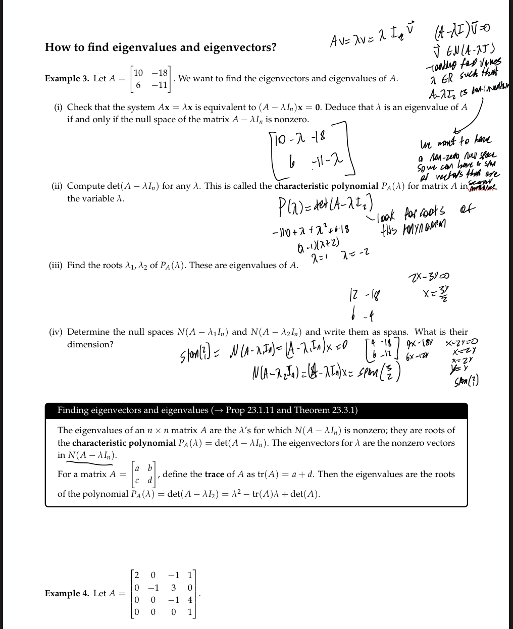
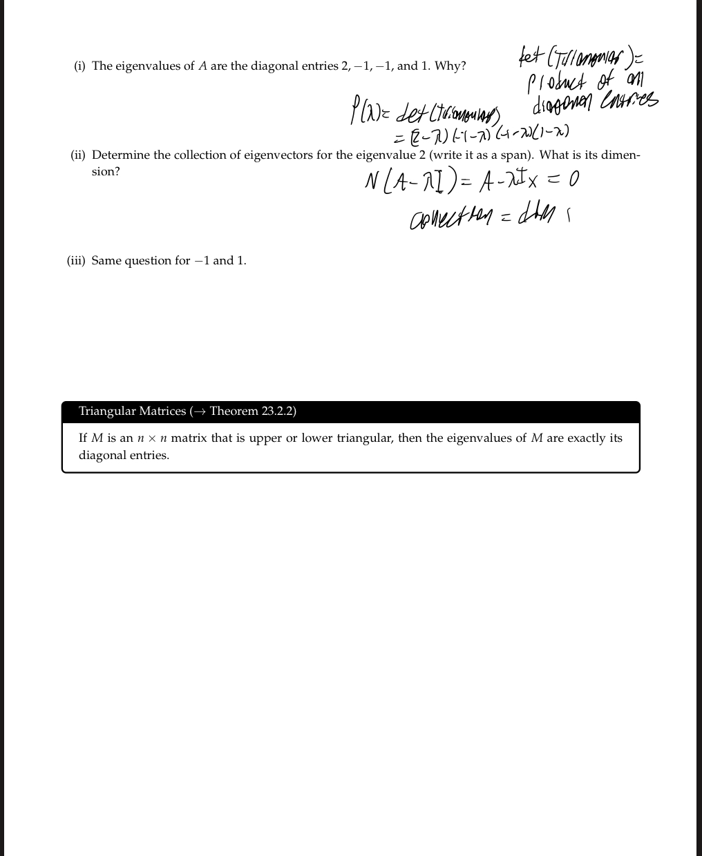
Chapter 24

Matrix Algebra

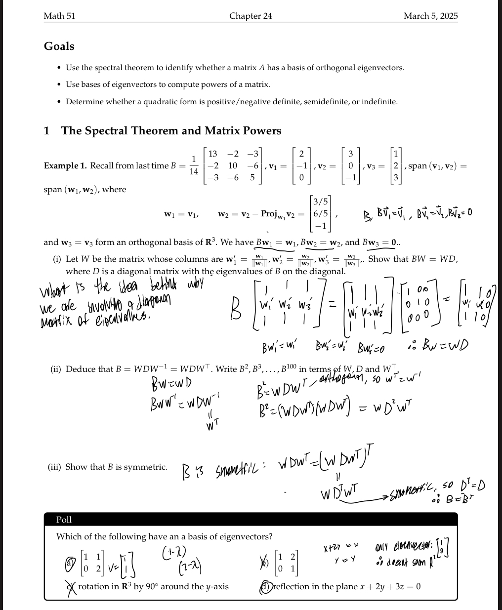
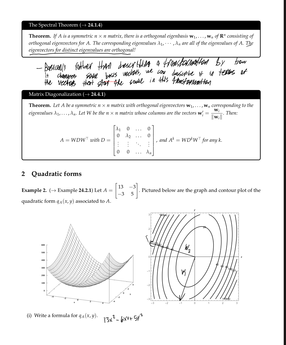
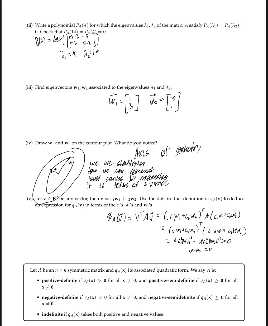
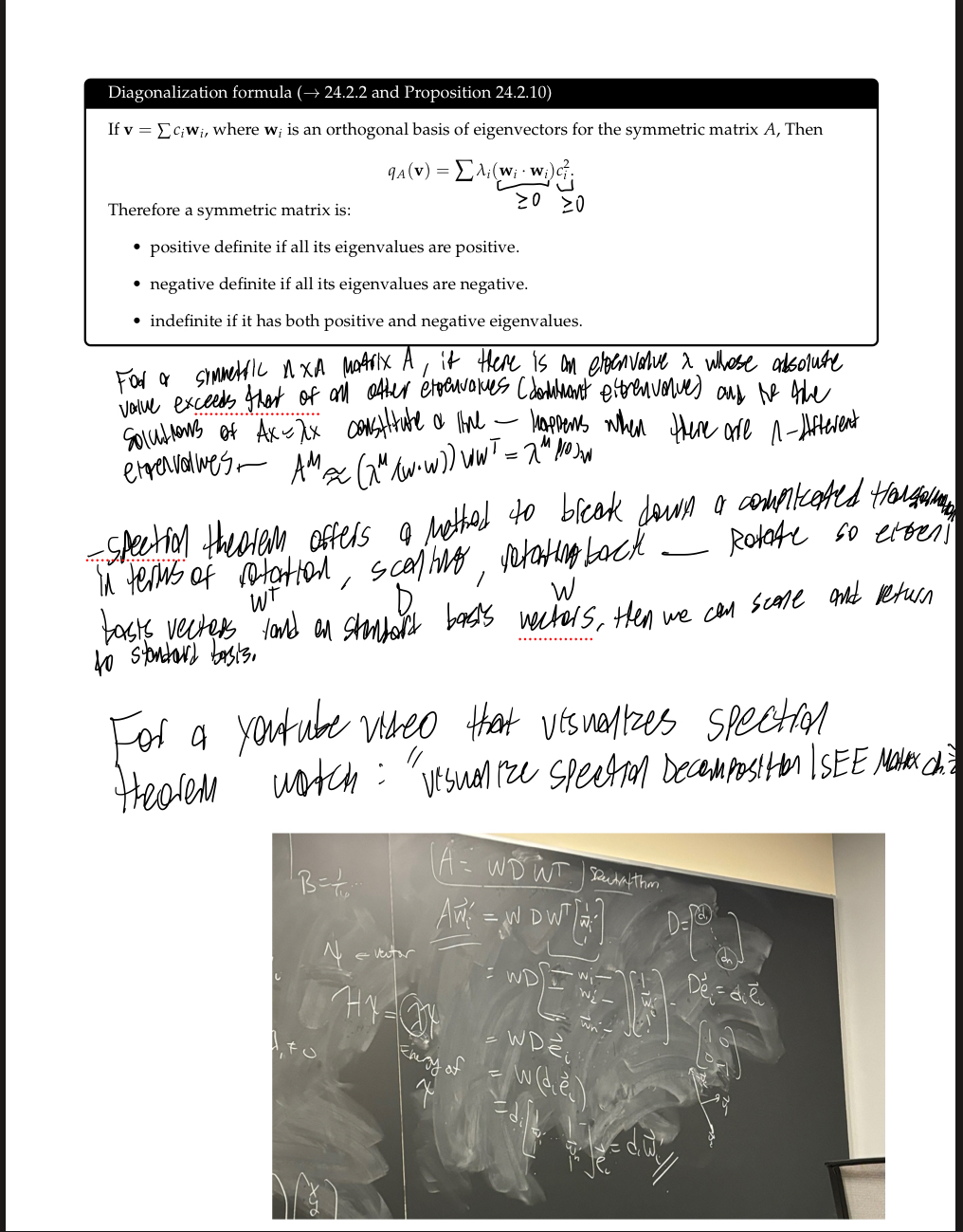
Chapter 25

Matrix Algebra