Infection Model
Absorbing Markov Chain Infection Model
A little introduction to stochastic processes through an infection model.
Overview
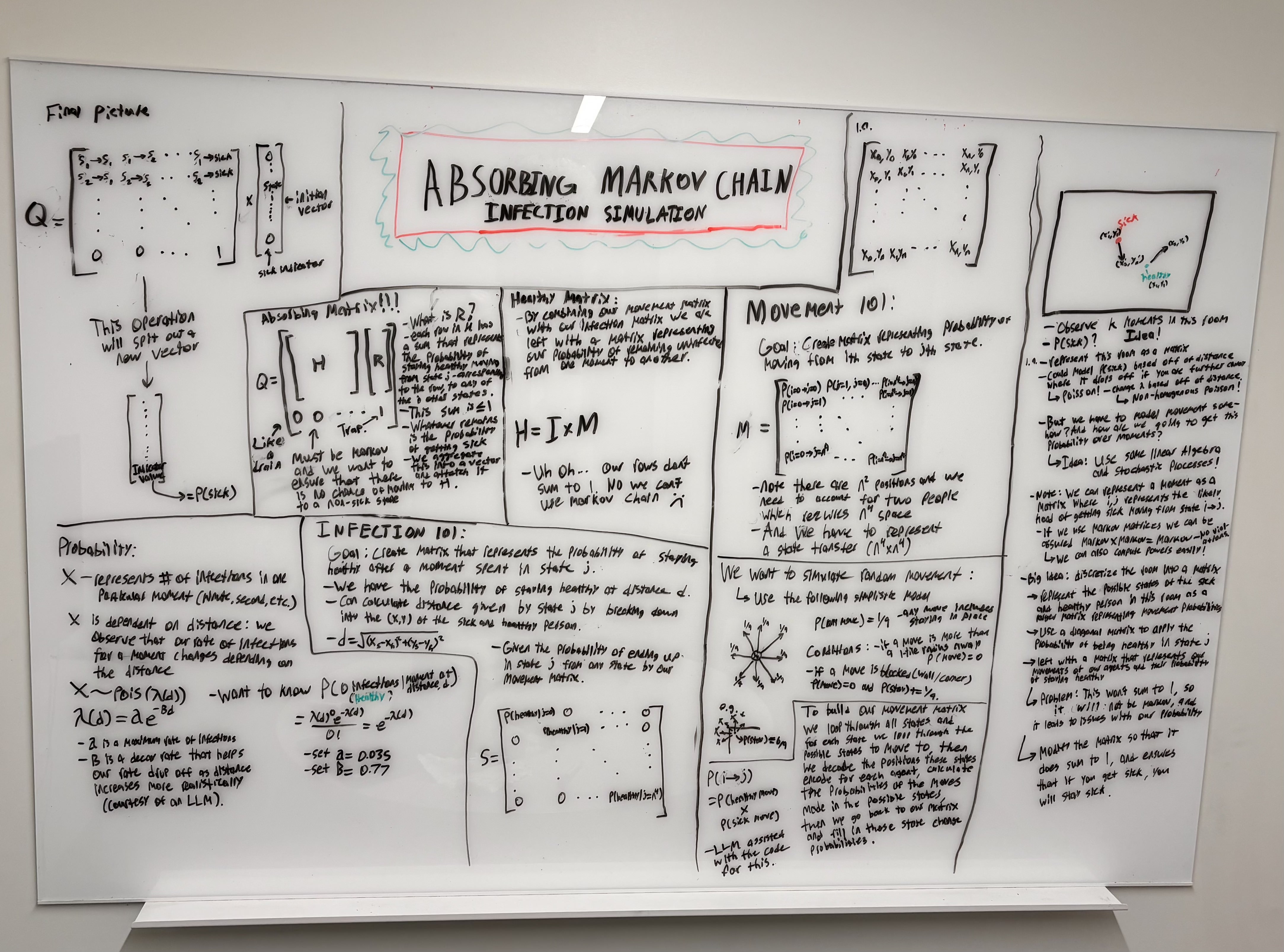
In this project I considered a situation in which there are two people in a room, one sick and one healthy, where the objective was to estimate the probability that the healthy person would become sick after some amount of time spent in the room. A few key assumptions were made when designing this problem: a) these individuals perform random walks in this room, b) the room is rectangular(can be represented spatially with a matrix), c) the probability of getting sick at any moment can be represented in terms of the distance between the sick and healthy person. The general idea of this project was to use my knowledge of probability and linear algebra to break down a seemingly difficult problem into one that could be solved quite easily with some clever tricks.
Approach
The first idea I had was to discretize the time and space of this situation, i.e. to represent each moment of the time interval discretely and represent each space in the room as an entry into a matrix. From there I would need to represent all the possible states of the room along with the positions of both the sick and healthy person into one composite matrix-M. We end up with a matrix where the ith row represents the ith state of all the possible states of the sick and healthy persons, and the jth column represents the possible transition states of both individuals from that ith state.
From there I had the idea that this could be used for a random walk representation, where the rows of this matrix sum to 1 in order to represent the idea that the probability that moving from any one state in the room to another should sum to 1. The next idea was to, as in the assumptions represent the probability of getting sick at any moment in terms of the distance between the sick and healthy person(which could be calculated thanks to the M matrix). This could be represented in terms of a diagonal matrix, P, where the entries are the probability of getting sick–or its compliment to represent the probability of staying healthy in the new jth state. I could then multiply these matrices together to get a matrix, Q, representing the probability of staying healthy in this room at a particular moment.
From there I realized that there were some issues, like my inability to keep track of sickness, ensure that sick people stay that way, and inability to take advantage of the nice properties of markov matrices. To approach this, I figured that I could represent my starting entry into this pseudo-random walk as just a vector with zeros except for the jth column representing the starting state–attached to this vector would be an extra entry to represent their probability of being sick.
From here I realized that if I consider the sum of the rows in my Q matrix, that represents the probability of staying healthy if you start in that ith state, and thus I could take the compliment of this sum and that would be my probability of getting sick in that state. Thus, I accumulate a vector that represents my probability of getting sick for each possible state, and I could attach this to my Q matrix to make it markov.
I still had the issue of potentially escaping the sick state, so I added a final row to the bottom of the matrix full of zeros except for the sick column which would be a 1, that way if an individual gets sick, then during the process of matrix-vector multiplication they would be ensured to stay sick. I was left with a markov matrix, which I could then take k-powers to represent k-moments of, and I could then multiply this by my initial state vector and look at the resulting final column entry which would represent the desired probability of getting sick after k-moments in the room.
Notes and Nuances
1. Infection Probability and the Non-Homogeneous Poisson Process
The probability of infection is not treated as a static constant; instead, it is modeled as a non-homogeneous Poisson process where the rate of infection, $\lambda$, is a function of the Euclidean distance ($d$) between the two individuals.
- The Rate Function: I used the formula $\lambda(d) = \alpha e^{-\beta d}$ to represent how viral shedding risk decays over space.
- Parameters: Following specific modeling constants, I set $\alpha = 0.035$ (the maximum expected infections per minute at zero distance) and $\beta = 0.77$ (the decay constant that dictates how quickly the risk drops as people move apart).
- Survival Logic: The entries in the diagonal matrix S (the “staying healthy” probabilities) are calculated as $P(X=0) = e^{-\lambda(d)}$, which represents the probability of zero infection events occurring during a discrete one-minute interval.
2. Movement Logic and Reflecting Boundaries
To ensure the room remains a closed system where probability is conserved, I implemented a Reflecting Boundary condition for the random walks.
- The 9-Option Walk: Each person has a base $1/9$ probability to move to any of the 8 adjacent tiles or stay put.
- Handling Walls: If a chosen move would take an individual out of the bounds of the $n \times n$ matrix, that move is “blocked”.
- Probability Absorption: Rather than losing that probability mass, the value of any blocked move is added back into the “Stay Put” probability. This ensures that the rows of the movement matrix M always sum exactly to 1, maintaining the Markov property.
3. Indexing Logic: Mapping Coordinates to the Matrix
To build the M matrix, I developed a consistent method to map the physical 2D positions of two people into a single 1D index for the matrix.
- Tile Encoding: For a room of width $n$, a person’s 2D position $(x, y)$ is collapsed into a single tile index: $T = (y-1) \times n + (x-1)$. This maps tiles from $0$ to $n^2-1$.
- State Encoding: Because the matrix must represent the joint state of both people, I combined their individual tile indices ($T_{sick}$ and $T_{healthy}$) into one master state index ($i$): $i = T_{sick} \times n^2 + T_{healthy}$.
- Decoding: This logic is reversible, allowing the simulation to “decode” any state index back into $(x, y)$ coordinates to calculate the Euclidean distance $d$ for the infection matrix.
4. State Space Complexity and Flaws ($n^4$)
While representing the room as an $n \times n$ grid is intuitive, the computational cost scales aggressively.
- Dimensions: Because a single state must track two independent positions, the state space is $n^2 \times n^2 = n^4$.
- The “N-to-the-Fourth” Problem: In a $9 \times 9$ room, we have 6,561 states, resulting in a matrix with over 43 million entries.
- Scalability: This is a significant flaw for larger environments; a $20 \times 20$ room would require a matrix with 25 billion entries, exceeding the memory capacity of most standard computers.
5. Binomial Model Extension
The model calculates the probability ($p$) for a single healthy person. To find the probability of infection for a group of $M$ healthy people:
- Independence: Assuming each person moves independently and the sick person is the only source of infection, we can use the Binomial Distribution.
- Formula: The probability that exactly $k$ people out of $M$ become sick is $P(X=k) = \binom{M}{k} p^k (1-p)^{M-k}$.
6. Alternative Solutions: Monte Carlo Simulation
An alternative to this linear algebra approach is a Monte Carlo Simulation.
- The Method: Instead of building a massive transition matrix, we would programmatically “walk” agents through the room thousands of times and record how often the healthy agent becomes sick based on the distance at each step.
- Trade-offs: While Monte Carlo is more memory-efficient and can handle larger rooms, it lacks the mathematical “exactness” of the Absorbing Markov Chain, which provides a precise analytical solution rather than an approximation based on trials.
Results & Visualization
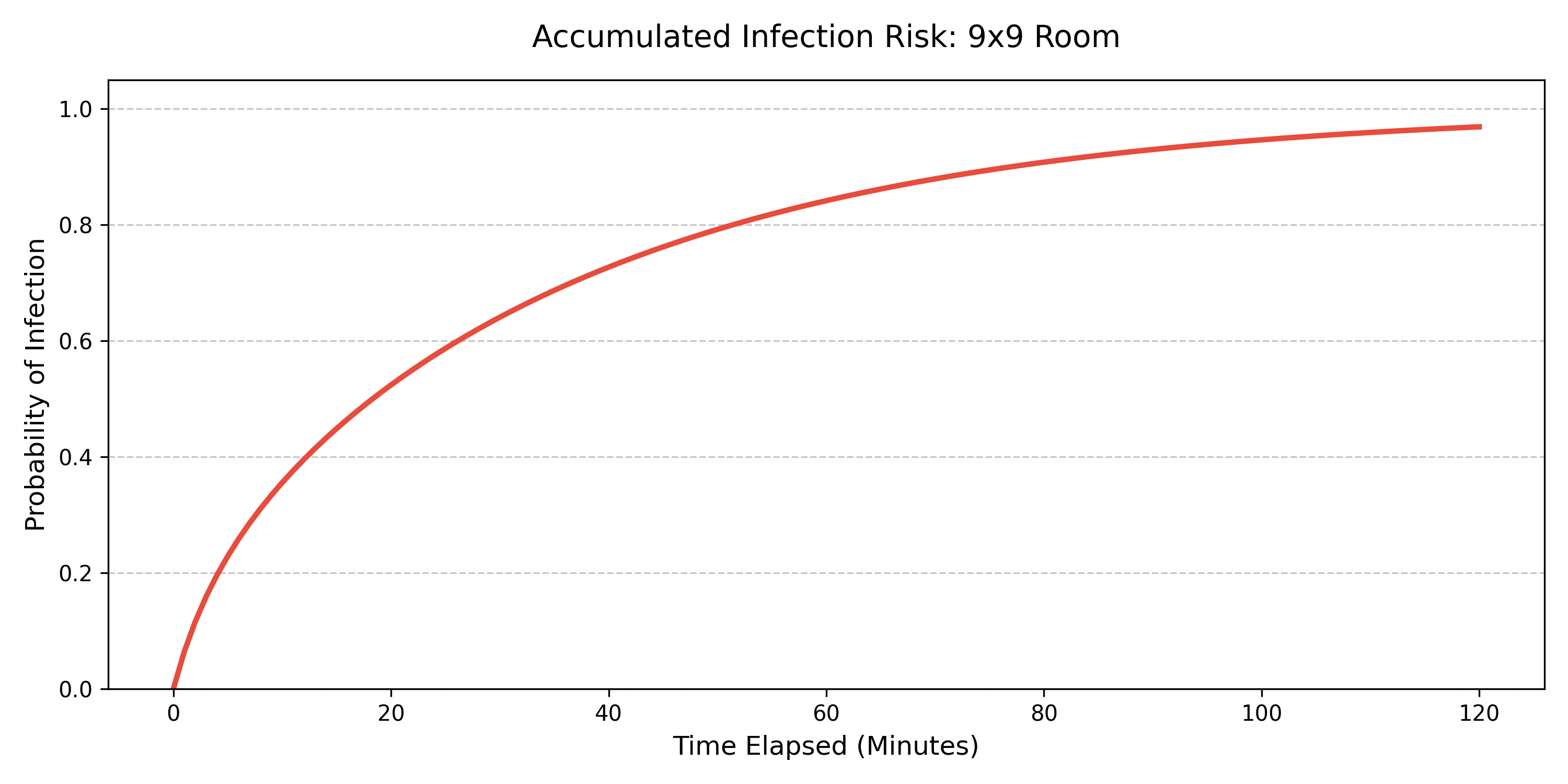
Below is the calculated infection risk over a 2-hour window in a 9x9 room. Notice the characteristic “absorbing” curve: as time progresses, the probability mass is trapped in the terminal state, ensuring that the cumulative risk strictly increases.
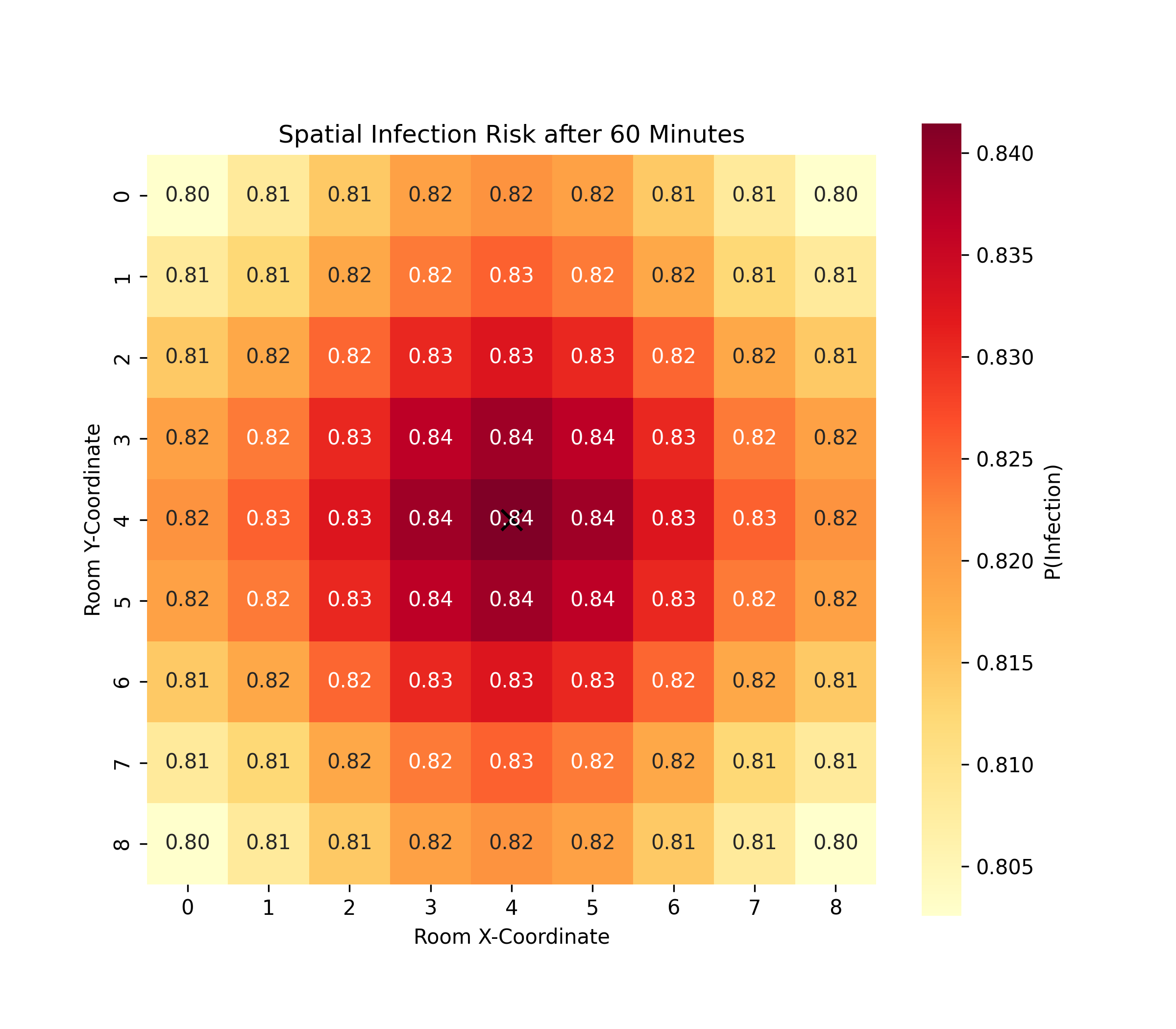
I also included a heat map to indicate how your position in the room affects your resulting probability of getting sick:
Full Source Code
To keep this page readable, I have collapsed the full 180-line Python implementation below. It includes the $O(n^4)$ matrix mapping logic and the reflecting boundary movement functions.
▶ Click to expand: model.py
import math
import numpy as np
import scipy.stats as stats
import numpy.linalg
import matplotlib.pyplot as plt
import os
import seaborn as sns

# --- I. Model Parameters ---
DECAY_RATE = 0.3
MAX_RATE = 0.1  # Use 0.035 for better results in 60 mins
P_BASE = 1.0 / 9.0


# --- II. Core Helper Functions ---

def eval_position(tile_index, width):
    """Maps a 1D tile index to 2D coordinates."""
    y = tile_index // width + 1
    x = tile_index % width + 1
    return x, y


def get_tile_index(x, y, width):
    """Maps 2D coordinates back to 1D tile index."""
    # x, y are 1-based. Index is 0-based.
    return (y - 1) * width + (x - 1)


def get_valid_moves_and_probs(start_index, width):
    """
    Returns a list of tuples: [(next_tile_index, probability), ...]
    This replaces looping through the whole grid.
    """
    moves = []
    x, y = eval_position(start_index, width)

    # Identify all neighbors (including self)
    neighbors = []
    blocked_count = 0

    # Check all 8 directions + stay (dx, dy from -1 to 1)
    for dx in [-1, 0, 1]:
        for dy in [-1, 0, 1]:
            if dx == 0 and dy == 0:
                continue  # We handle 'Stay' separately at the end

            nx, ny = x + dx, y + dy

            # Check if wall
            if nx < 1 or nx > width or ny < 1 or ny > width:
                blocked_count += 1
            else:
                # Valid neighbor
                n_idx = get_tile_index(nx, ny, width)
                neighbors.append(n_idx)

    # 1. Add probability for moving to valid neighbors
    for n_idx in neighbors:
        moves.append((n_idx, P_BASE))

    # 2. Add probability for Staying Put (Base + Absorbed Wall Bumps)
    stay_prob = P_BASE + (blocked_count * P_BASE)
    moves.append((start_index, stay_prob))

    return moves


# --- III. Matrix Constructors (Optimized) ---

def construct_mvmt_mtx(room_width):
    """
    Optimized construction.
    Instead of 43 million loops, we only process valid moves (~500k ops).
    """
    n = room_width ** 2
    num_states = n * n
    m = np.zeros((num_states, num_states))

    # 1. Loop through all Starting States (i)
    for t_s in range(n):
        # Pre-calculate valid moves for Sick person from this tile
        moves_s = get_valid_moves_and_probs(t_s, room_width)

        for t_h in range(n):
            # Pre-calculate valid moves for Healthy person from this tile
            moves_h = get_valid_moves_and_probs(t_h, room_width)

            # Current State Index i
            i = (t_s * n) + t_h

            # 2. Iterate ONLY over valid next steps (j)
            # This replaces the inner 2 loops (81*81 iterations) with just ~9*9 iterations
            for (next_s, prob_s) in moves_s:
                for (next_h, prob_h) in moves_h:
                    # Target State Index j
                    j = (next_s * n) + next_h

                    # Set Probability
                    m[i, j] = prob_s * prob_h

    return m


def calc_distance(sick_index, healthy_index, room_width):
    sick_pos = eval_position(sick_index, room_width)
    healthy_pos = eval_position(healthy_index, room_width)
    return math.sqrt(((sick_pos[0] - healthy_pos[0]) ** 2) + ((sick_pos[1] - healthy_pos[1]) ** 2))


def prob_healthy(distance):
    lam = MAX_RATE * (math.e ** (-1 * DECAY_RATE * distance))
    # Poisson PMF at 0 is just e^-lambda
    return math.exp(-lam)


def construct_infect_mtx(width):
    n = width ** 2
    num_states = n * n
    s = np.zeros((num_states, num_states))
    for i in range(num_states):
        t_s = i // n
        t_h = i % n
        distance = calc_distance(t_s, t_h, width)
        p_survival = prob_healthy(distance)
        s[i, i] = p_survival
    return s


def calculate_transition_matrix(m, s, width):
    n = width * width
    num_states = n * n

    # Q = M x S
    Q = m @ s

    # Calculate Leak Vector R
    R = 1.0 - np.sum(Q, axis=1)

    n_total = num_states + 1
    P = np.zeros((n_total, n_total))

    # Fill P
    P[:num_states, :num_states] = Q
    P[:num_states, num_states] = R  # R is flat array, fits into column
    P[num_states, num_states] = 1.0

    return P


def simulate_room(width, sick_start_tile_index, healthy_start_tile_index, time_steps=60):
    print(f"Constructing matrices for {width}x{width} room...")
    n = width * width
    num_states = n * n
    n_total = num_states + 1

    m = construct_mvmt_mtx(width)
    s = construct_infect_mtx(width)
    P = calculate_transition_matrix(m, s, width)

    print("Matrices built. Simulating steps...")

    starting_state_index = sick_start_tile_index * n + healthy_start_tile_index
    v0 = np.zeros(n_total)
    v0[starting_state_index] = 1.0

    P_k = np.linalg.matrix_power(P, time_steps)
    v_k = v0 @ P_k

    return v_k[-1]


def generate_visual(width, s_idx, h_idx, time_steps=120):
    print("Generating visualization data...")
    n = width * width
    num_states = n * n

    # 1. Build the matrix once
    m = construct_mvmt_mtx(width)
    s = construct_infect_mtx(width)
    P = calculate_transition_matrix(m, s, width)

    # 2. Track probability over time
    starting_state_index = s_idx * n + h_idx
    v = np.zeros(num_states + 1)
    v[starting_state_index] = 1.0

    time_axis = []
    prob_axis = []

    for t in range(time_steps + 1):
        time_axis.append(t)
        prob_axis.append(v[-1])  # The last entry is our 'Sick' state
        v = v @ P  # Step forward by 1 minute

    # 3. Create a professional plot
    plt.style.use('seaborn-v0_8-muted')  # Clean, modern look
    plt.figure(figsize=(10, 5))
    plt.plot(time_axis, prob_axis, color='#e74c3c', linewidth=2.5, label='P(Infected)')

    plt.title(f'Accumulated Infection Risk: {width}x{width} Room', fontsize=14, pad=15)
    plt.xlabel('Time Elapsed (Minutes)', fontsize=12)
    plt.ylabel('Probability of Infection', fontsize=12)
    plt.ylim(0, 1.05)
    plt.grid(axis='y', linestyle='--', alpha=0.7)
    plt.tight_layout()

    os.makedirs('static/images', exist_ok=True)

    plt.savefig('static/images/infection_plot.png', dpi=300)
    # Note: Make sure the directory 'static/images/' exists first
    print("Saved plot to static/images/infection_plot.png")
    plt.show()


def generate_heatmap(width, s_idx, time_steps=60):
    print(f"Generating {width}x{width} Heat Map (this may take a moment)...")

    # 1. Build the matrix once (the expensive part)
    m = construct_mvmt_mtx(width)
    s = construct_infect_mtx(width)
    P = calculate_transition_matrix(m, s, width)
    P_k = np.linalg.matrix_power(P, time_steps)

    n = width * width
    heatmap_data = np.zeros((width, width))

    # 2. Test every possible starting position for the healthy person
    for h_idx in range(n):
        v0 = np.zeros(n ** 2 + 1)
        start_state = (s_idx * n) + h_idx
        v0[start_state] = 1.0

        # Multiply by the powered matrix
        v_k = v0 @ P_k
        prob = v_k[-1]

        # Map 1D index back to 2D for the plot
        x_h, y_h = eval_position(h_idx, width)
        heatmap_data[y_h - 1, x_h - 1] = prob

    # 3. Plotting
    plt.figure(figsize=(8, 7))
    # 'YlOrRd' is a great color map for risk (Yellow to Red)
    ax = sns.heatmap(heatmap_data, annot=True, fmt=".2f", cmap='YlOrRd',
                     square=True, cbar_kws={'label': 'P(Infection)'})

    # Mark where the sick person is
    x_s, y_s = eval_position(s_idx, width)
    plt.scatter(x_s - 0.5, y_s - 0.5, marker='x', color='black', s=100, label='Sick Person Start')

    plt.title(f'Spatial Infection Risk after {time_steps} Minutes')
    plt.xlabel('Room X-Coordinate')
    plt.ylabel('Room Y-Coordinate')

    os.makedirs('static/images', exist_ok=True)
    plt.savefig('static/images/infection_heatmap.png', dpi=300)
    print("Success! Heat map saved to static/images/infection_heatmap.png")

def main():
    # Example: 9x9 room.
    # Sick person starts at Tile 3 (Left Wall).
    # Healthy person starts at Tile 40 (Center).
    prob = simulate_room(width=9, sick_start_tile_index=40, healthy_start_tile_index=40, time_steps=600)

    print(f"Probability of infection: {prob:.4f}")
    return 0


if __name__ == "__main__":
    generate_visual(width=9, s_idx=40, h_idx=40)