Real-Analysis Notes
Overview
Here are my notes for my course in real-analysis. The course textbook was Ross-Elementary Analysis. The course covered up until uniform convergence and the Weierstrass M-test. I supplemented some of the gaps in content with Stephen Abbott’s Understanding Analysis textbook for concepts such as measure and point-set topology etc.
Chapter 1: The Real Numbers
Quick Overview
Analysis begins with a rigorous construction of the number systems we use. While Calculus relies on computational rules, Analysis relies on the axiomatic properties of the set of real numbers, denoted $\mathbf{R}$. This chapter builds $\mathbf{R}$ from the ground up, starting with the natural numbers ($\mathbf{N}$) and moving through the field and order axioms, culminating in the Completeness Axiom—the property that distinguishes $\mathbf{R}$ from the rational numbers ($\mathbf{Q}$) and allows for the existence of limits.
1.1 The Natural Numbers and Induction
The Peano Axioms
The natural numbers $\mathbf{N} = {1, 2, 3, \dots}$ are defined not by listing them, but by a set of axioms known as the Peano Axioms. These provide a rigorous foundation for counting and arithmetic.
Definition 1.1.1 (Peano Axioms): The set $\mathbf{N}$ satisfies the following properties:
- $1 \in \mathbf{N}$.
- For every $n \in \mathbf{N}$, there exists a unique successor element $S(n) \in \mathbf{N}$.
- $1$ is not the successor of any element in $\mathbf{N}$ (i.e., $S(n) \neq 1$ for all $n$).
- The successor function is injective: If $S(n) = S(m)$, then $n = m$.
- Axiom of Induction: If a subset $K \subseteq \mathbf{N}$ contains $1$, and if the property “$k \in K$ implies $S(k) \in K$” holds, then $K = \mathbf{N}$.
Mathematical Induction
The fifth axiom gives rise to the Principle of Mathematical Induction, which is our primary tool for proving statements indexed by natural numbers.
Theorem 1.1.2 (Principle of Mathematical Induction): Let $P(n)$ be a statement for each $n \in \mathbf{N}$. If:
- Base Case: $P(1)$ is true.
- Inductive Step: For every $k \in \mathbf{N}$, if $P(k)$ is true, then $P(k+1)$ is true. Then $P(n)$ is true for all $n \in \mathbf{N}$.
1.2 Algebraic Properties and the Rational Zeros Theorem
The real numbers form a Field, satisfying the standard axioms of commutativity, associativity, distributivity, and the existence of identities ($0, 1$) and inverses. However, identifying which numbers belong to $\mathbf{Q}$ (Rationals) versus $\mathbf{R} \setminus \mathbf{Q}$ (Irrationals) requires specific tools.
Theorem 1.2.1 (The Rational Zeros Theorem): Suppose that $c_n x^n + c_{n-1} x^{n-1} + \dots + c_1 x + c_0 = 0$ is a polynomial equation with integer coefficients ($c_i \in \mathbf{Z}$). If a rational number $r = p/q$ (where $p$ and $q$ are coprime integers) is a solution to this equation, then:
- $p$ divides the constant term $c_0$ ($p | c_0$).
- $q$ divides the leading coefficient $c_n$ ($q | c_n$).
Application: The Irrationality of $\sqrt{2}$
The Rational Zeros Theorem provides a direct method to prove that certain numbers are not rational.
Corollary 1.2.2 ($\sqrt{2} \notin \mathbf{Q}$): There is no rational number $r$ such that $r^2 = 2$. Proof: Consider the polynomial $x^2 - 2 = 0$.
- The coefficients are integers: $c_2 = 1, c_1 = 0, c_0 = -2$.
- By the Rational Zeros Theorem, any rational root $p/q$ must satisfy:
- $p$ divides $-2$ (so $p \in {\pm 1, \pm 2}$).
- $q$ divides $1$ (so $q \in {\pm 1}$).
- The only possible rational candidates are $\pm 1$ and $\pm 2$.
- Testing these candidates:
- $(\pm 1)^2 - 2 = -1 \neq 0$
- $(\pm 2)^2 - 2 = 2 \neq 0$
- Since none of the candidates are roots, the equation $x^2 - 2 = 0$ has no rational solutions. Thus, $\sqrt{2}$ is irrational.
1.3 The Order Properties of $\mathbf{R}$
In addition to being a field, $\mathbf{R}$ is an Ordered Set. This ordering allows us to compare the size of real numbers and gives rise to the concept of positivity.
Definition 1.3.1 (Order Axioms): There exists a non-empty subset $\mathbf{P} \subseteq \mathbf{R}$, called the set of positive real numbers, satisfying:
- Closure under Addition: If $a, b \in \mathbf{P}$, then $a+b \in \mathbf{P}$.
- Closure under Multiplication: If $a, b \in \mathbf{P}$, then $ab \in \mathbf{P}$.
- Trichotomy Property: For any $a \in \mathbf{R}$, exactly one of the following holds:
- $a \in \mathbf{P}$
- $a = 0$
- $-a \in \mathbf{P}$
Definition 1.3.2 (Inequalities): We define inequalities based on $\mathbf{P}$:
- $a < b$ if $b - a \in \mathbf{P}$.
- $a \leq b$ if $a < b$ or $a = b$.
Theorem 1.3.3 (Properties of Inequalities):
- Transitivity: If $a < b$ and $b < c$, then $a < c$.
- Addition: If $a < b$, then $a+c < b+c$.
- Multiplication:
- If $a < b$ and $c > 0$, then $ac < bc$.
- If $a < b$ and $c < 0$, then $ac > bc$ (Inequality flips).
- Squares: If $a \neq 0$, then $a^2 > 0$. Consequently, $1 > 0$.
Absolute Value
The order axioms allow us to define the magnitude of a number.
Definition 1.3.4 (Absolute Value): For any $a \in \mathbf{R}$, the absolute value $|a|$ is defined as: $$|a| = \begin{cases} a & \text{if } a \geq 0 \ -a & \text{if } a < 0 \end{cases}$$
Theorem 1.3.5 (The Triangle Inequality): For any $a, b \in \mathbf{R}$: $$|a + b| \leq |a| + |b|$$ Corollary: $||a| - |b|| \leq |a - b|$.
1.4 The Completeness Axiom
The Rational numbers ($\mathbf{Q}$) satisfy all the Field and Order axioms listed above. However, $\mathbf{Q}$ has “gaps” (e.g., as proved in Section 1.2, $\sqrt{2} \notin \mathbf{Q}$). The Completeness Axiom fills these gaps and is the defining property of $\mathbf{R}$.
Definition 1.4.1 (Upper and Lower Bounds): Let $S$ be a non-empty subset of $\mathbf{R}$.
- $S$ is bounded above if there exists $b \in \mathbf{R}$ such that $s \leq b$ for all $s \in S$. Such a $b$ is called an upper bound.
- $S$ is bounded below if there exists $w \in \mathbf{R}$ such that $w \leq s$ for all $s \in S$. Such a $w$ is called a lower bound.
Definition 1.4.2 (Supremum and Infimum):
- Supremum ($\sup S$): The least upper bound of $S$. A number $\alpha$ is the supremum if:
- $\alpha$ is an upper bound of $S$.
- If $\beta$ is any other upper bound of $S$, then $\alpha \leq \beta$.
- Infimum ($\inf S$): The greatest lower bound of $S$. A number $\gamma$ is the infimum if:
- $\gamma$ is a lower bound of $S$.
- If $\beta$ is any other lower bound of $S$, then $\gamma \geq \beta$.
Axiom 1.4.3 (The Completeness Axiom of $\mathbf{R}$): Every non-empty set of real numbers that is bounded above has a supremum in $\mathbf{R}$.
(Note: It can be proved that every non-empty set bounded below has an infimum in $\mathbf{R}$ as a consequence of this axiom.)
Lemma 1.4.4 (Approximation Property for Supremum): This is a critical tool for proofs. A number $\alpha$ is the supremum of $S$ if and only if:
- $s \leq \alpha$ for all $s \in S$.
- For any $\epsilon > 0$, there exists some element $s_\epsilon \in S$ such that $\alpha - \epsilon < s_\epsilon$.
1.5 Consequences of Completeness
The Completeness Axiom leads to two fundamental properties of the Real number line used throughout analysis.
Theorem 1.5.1 (The Archimedean Property): For any $x \in \mathbf{R}$, there exists a natural number $n \in \mathbf{N}$ such that $n > x$. Implication: The set $\mathbf{N}$ is not bounded above in $\mathbf{R}$.
Theorem 1.5.2 (Density of $\mathbf{Q}$ in $\mathbf{R}$): For any two real numbers $x$ and $y$ with $x < y$, there exists a rational number $r \in \mathbf{Q}$ such that $x < r < y$. Intuition: Between any two real numbers, no matter how close, there is always a fraction.
Theorem 1.5.3 (Existence of $\sqrt{2}$): There exists a unique positive real number $x$ such that $x^2 = 2$. (This proof utilizes the Completeness Axiom by defining the set $S = {s \in \mathbf{R} : s \geq 0, s^2 < 2}$ and showing that $\sup S$ must be exactly $\sqrt{2}$.)
Chapter 2: Sequences and Series
Quick Overview
Chapter 2 shifts from the static properties of real numbers to the dynamic concept of Sequences. The central goal is to rigorously define “convergence” using the $\epsilon-N$ quantifier logic, moving away from the vague “gets closer to” language of Calculus. We also explore intrinsic properties like monotonicity and compactness (Bolzano-Weierstrass) to determine convergence without knowing the limit beforehand.
2.1 The Limit of a Sequence
Definition of Convergence
The rigorous definition of a limit is the cornerstone of analysis. It quantifies the idea that eventually, the sequence stays within an arbitrarily small error margin.
Definition 2.2.3 (Convergence): A sequence $(a_n)$ converges to a real number $a$ if, for every $\epsilon > 0$, there exists a natural number $N \in \mathbf{N}$ such that for all $n \geq N$: $$|a_n - a| < \epsilon$$ .
Theorem 2.2.7 (Uniqueness of Limits): If a sequence converges, its limit is unique. That is, if $(a_n) \to a$ and $(a_n) \to b$, then $a = b$.
2.2 Algebraic and Order Limit Theorems
We establish rules to calculate limits of complex expressions without using the $\epsilon-N$ definition every time.
Theorem 2.3.2 (Boundedness): Every convergent sequence is bounded. Note: The converse is false (e.g., $(-1)^n$), which motivates the Bolzano-Weierstrass theorem later.
Theorem 2.3.3 (Algebraic Limit Theorem): Let $\lim a_n = a$ and $\lim b_n = b$. Then:
- Sum: $\lim(a_n + b_n) = a + b$
- Scalar Product: $\lim(ca_n) = ca$
- Product: $\lim(a_n b_n) = ab$
- Quotient: $\lim(a_n / b_n) = a/b$ (provided $b \neq 0$ and $b_n \neq 0$) .
Theorem 2.3.4 (Order Limit Theorem): If $a_n \to a$, $b_n \to b$, and $a_n \leq b_n$ for all $n$, then $a \leq b$.
Theorem 2.3.5 (Squeeze Theorem): If $a_n \leq x_n \leq b_n$ for all $n$, and $\lim a_n = \lim b_n = \ell$, then $\lim x_n = \ell$.
Theorem 2.3.6 (Comparison Lemma for Absolute Values): If $|a_n| \to 0$, then $a_n \to 0$. This is often useful for sequences with oscillating signs.
2.3 Monotone Convergence and Infinite Limits
Definition 2.4.1 (Monotonicity): A sequence is monotone if it is either non-decreasing ($a_{n+1} \geq a_n$) or non-increasing ($a_{n+1} \leq a_n$).
Theorem 2.4.2 (Monotone Convergence Theorem): If a sequence is monotone and bounded, then it converges.
- If increasing and bounded above, it converges to $\sup{a_n}$.
- If decreasing and bounded below, it converges to $\inf{a_n}$. .
Definition 2.4.3 (Infinite Limits): We say $\lim a_n = +\infty$ if for every $M > 0$, there exists $N \in \mathbf{N}$ such that $a_n > M$ for all $n \geq N$. (This is technically “divergence”, but a specific kind).
2.4 Subsequences and Compactness
Definition 2.5.1 (Subsequence): Let $(n_k)$ be a strictly increasing sequence of natural numbers ($n_1 < n_2 < \dots$). Then $(a_{n_k})$ is a subsequence of $(a_n)$.
Theorem 2.5.2 (Subsequence Limits): If a sequence $(a_n)$ converges to $a$, then every subsequence $(a_{n_k})$ also converges to $a$.
Theorem 2.5.5 (Bolzano-Weierstrass Theorem): Every bounded sequence contains a convergent subsequence. Significance: This is a crucial “compactness” result. Even if a sequence oscillates (like $(-1)^n$), if it stays bounded, we can always find a “nice” path through it that converges.
My Proof of Bolzano-Weierstrass
Most textbooks use the Nested Interval Property. I have derived the proof using a “Divide and Conquer” interval halving strategy:
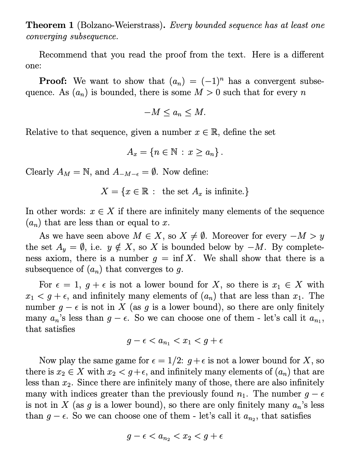
Key Insight: Since the sequence is bounded, it lives in some interval $I_0$. Split $I_0$ in half. By the Pigeonhole Principle, one half must contain infinitely many points. Call this $I_1$. Repeat this process to get a nested sequence $I_k$ whose size shrinks to 0. By the Nested Interval Property, there is a single point $x$ in the intersection, which is the limit of our subsequence.
Theorem 2.5.3 (Nested Interval Property): For a sequence of closed intervals $I_n = [a_n, b_n]$ such that $I_{n+1} \subseteq I_n$ for all $n$, the intersection $\bigcap_{n=1}^{\infty} I_n$ is non-empty. If length$(I_n) \to 0$, the intersection contains a unique point.
2.6 Cauchy Sequences and Limit Superior and Inferior
Definition 2.6.1 (Cauchy Sequence): A sequence $(a_n)$ is a Cauchy sequence if for every $\epsilon > 0$, there exists $N \in \mathbf{N}$ such that for all $n, m \geq N$: $$|a_n - a_m| < \epsilon$$ Intuition: The terms eventually get arbitrarily close to each other, independent of any limit $L$.
Theorem 2.6.4 (Cauchy Criterion): A sequence converges if and only if it is a Cauchy sequence.
- $(\implies)$ Easy (Triangle Inequality).
- $(\impliedby)$ Hard (Requires Completeness of $\mathbf{R}$).
Motivation
Not all bounded sequences converge (e.g., $a_n = (-1)^n$). However, bounded sequences always stay within a certain range. $\limsup$ and $\liminf$ allow us to quantify the “upper” and “lower” limits of that oscillation range. Unlike the standard limit, $\limsup$ and $\liminf$ always exist for any bounded sequence.
Definitions
Let $(a_n)$ be a bounded sequence. We define the “tail” supremum $v_n$ as the supremum of everything after index $n$: $$v_n = \sup {a_k : k \geq n}$$ Since the set of terms shrinks as $n$ increases, the sequence $(v_n)$ is monotone decreasing. By the Monotone Convergence Theorem, it must converge.
Definition 2.9.1 (Limit Superior): $$\limsup_{n \to \infty} a_n = \lim_{n \to \infty} (\sup {a_k : k \geq n})$$ Intuition: This is the limit of the “ceilings” of the sequence tails.
Definition 2.9.2 (Limit Inferior): Similarly, let $u_n = \inf {a_k : k \geq n}$. This sequence is monotone increasing. $$\liminf_{n \to \infty} a_n = \lim_{n \to \infty} (\inf {a_k : k \geq n})$$ Intuition: This is the limit of the “floors” of the sequence tails.
Key Properties and Theorems
Theorem 2.9.3 (Subsequential Characterization): The $\limsup a_n$ is the largest subsequential limit of $(a_n)$. The $\liminf a_n$ is the smallest subsequential limit of $(a_n)$. Example: For $a_n = (-1)^n$, the subsequential limits are $1$ and $-1$.
- $\limsup a_n = 1$
- $\liminf a_n = -1$
Theorem 2.9.4 (Convergence Criterion): A sequence $(a_n)$ converges if and only if its upper and lower limits are equal. $$\lim_{n \to \infty} a_n = L \iff \limsup a_n = \liminf a_n = L$$
Theorem 2.9.5 (Order Property): For any sequence, we always have the ordering: $$\inf {a_n} \leq \liminf a_n \leq \limsup a_n \leq \sup {a_n}$$
Application
These tools are often used in the Ratio Test and Root Test for series (Chapter 3), where the limit itself might not exist, but the $\limsup$ provides a strict upper bound on growth.
2.7 Special Limits and The Number $e$
The Definition of $e$
A classic application of the Monotone Convergence Theorem is the definition of Euler’s number.
Theorem 2.7.1 (The Limit $e$): Consider the sequence $e_n = (1 + \frac{1}{n})^n$.
- Monotonicity: By using the Binomial Theorem (or Bernoulli’s Inequality), one can show that $e_{n+1} \geq e_n$ for all $n$.
- Boundedness: One can show that $e_n < 3$ for all $n$. By the Monotone Convergence Theorem, the sequence converges. We define the limit to be $e$: $$e = \lim_{n \to \infty} \left(1 + \frac{1}{n}\right)^n$$
Bernoulli’s Inequality
A crucial tool for proving limits involving exponents (like the one above) is Bernoulli’s Inequality.
Theorem 2.7.2 (Bernoulli’s Inequality): For any $x > -1$ and $n \in \mathbf{N}$: $$(1+x)^n \geq 1 + nx$$
Ratio Test for Sequences
While typically associated with series, the Ratio Test is also a theorem for sequences, useful for determining if a sequence converges to 0.
Theorem 2.7.3 (Ratio Test for Sequences): Let $(a_n)$ be a sequence of positive terms such that $\lim (a_{n+1}/a_n) = L$.
- If $L < 1$, then $\lim a_n = 0$.
- If $L > 1$, then $\lim a_n = +\infty$ (diverges).
- If $L = 1$, the test is inconclusive.
Common Special Limits
Using the Squeeze Theorem and Bernoulli’s Inequality, we establish these standard results used in future chapters:
The “n-th root of n”: $$\lim_{n \to \infty} n^{1/n} = 1$$ Proof Strategy: Let $x_n = n^{1/n} - 1$. Then $n = (1+x_n)^n$. Using the binomial expansion, we can “squeeze” $x_n$ to 0.
Powers of real numbers: If $|x| < 1$, then $\lim_{n \to \infty} x^n = 0$.
2.8 Infinite Series (Sections 14-16)
Definition 2.8.1 (Infinite Series): An infinite series $\sum_{n=1}^{\infty} a_n$ is defined as the limit of the sequence of partial sums $(s_m)$, where $s_m = \sum_{n=1}^{m} a_n$. If $\lim_{m \to \infty} s_m = S$, the series converges to $S$.
Theorem 2.8.2 (The Geometric Series Test): A geometric series $\sum_{n=0}^{\infty} r^n$ converges if and only if $|r| < 1$.
- If $|r| < 1$, the sum is $\frac{1}{1-r}$.
- If $|r| \geq 1$, the series diverges. .
Theorem 2.8.3 (The Cauchy Criterion for Series): A series $\sum a_n$ converges if and only if for every $\epsilon > 0$, there exists $N \in \mathbf{N}$ such that for all $m > n \geq N$: $$|s_m - s_n| = \left| \sum_{k=n+1}^{m} a_k \right| < \epsilon$$ .
Theorem 2.8.4 (The Divergence Test / $n$-th Term Test): If $\sum a_n$ converges, then $\lim_{n \to \infty} a_n = 0$.
- Contrapositive: If $\lim a_n \neq 0$, then $\sum a_n$ diverges.
- Warning: The harmonic series $\sum 1/n$ diverges even though $1/n \to 0$.
Theorem 2.8.5 (Algebraic Properties): If $\sum a_n = A$ and $\sum b_n = B$, then $\sum (ca_n + b_n) = cA + B$.
Theorem 2.8.6 (Convergence of Non-Negative Series): If $a_n \geq 0$ for all $n$, then the partial sums $(s_m)$ are increasing. The series $\sum a_n$ converges if and only if the sequence of partial sums is bounded above.
Theorem 2.8.7 (The Comparison Test): Let $0 \leq a_n \leq b_n$ for all $n$.
- If $\sum b_n$ converges, then $\sum a_n$ converges.
- If $\sum a_n$ diverges, then $\sum b_n$ diverges. .
Theorem 2.8.8 (The Limit Comparison Test): Suppose $a_n > 0$ and $b_n > 0$ and $\lim_{n \to \infty} \frac{a_n}{b_n} = L$.
- If $0 < L < \infty$, then $\sum a_n$ and $\sum b_n$ either both converge or both diverge.
- This allows us to compare “messy” series to simple $p$-series by looking at their dominant terms.
Theorem 2.8.9 (The $p$-Series Test): The series $\sum_{n=1}^{\infty} \frac{1}{n^p}$ converges if and only if $p > 1$.
- If $p \leq 1$, the series diverges. (This generalizes the Harmonic Series, where $p=1$).
Theorem 2.8.10 (Cauchy Condensation Test): Suppose $(a_n)$ is non-increasing and non-negative ($a_1 \geq a_2 \geq \dots \geq 0$). Then the series $\sum_{n=1}^{\infty} a_n$ converges if and only if the “condensed” series $\sum_{k=0}^{\infty} 2^k a_{2^k}$ converges.
- Note: This is often used to prove the divergence of the Harmonic Series and the $p$-series test.
Theorem 2.8.11 (Alternating Series Test / Leibniz Test): Let $(a_n)$ be a decreasing sequence of positive numbers ($a_1 \geq a_2 \geq \dots > 0$) such that $\lim a_n = 0$. Then the alternating series $\sum_{n=1}^{\infty} (-1)^{n+1} a_n$ converges.
- Example: The Alternating Harmonic Series $\sum \frac{(-1)^{n+1}}{n}$ converges, even though $\sum \frac{1}{n}$ diverges.
Definition 2.8.12 (Absolute vs. Conditional Convergence):
- $\sum a_n$ converges absolutely if $\sum |a_n|$ converges.
- $\sum a_n$ converges conditionally if $\sum a_n$ converges but $\sum |a_n|$ diverges.
Theorem 2.8.13 (Absolute Convergence Theorem): If a series converges absolutely, it converges. $$\text{If } \sum |a_n| < \infty \implies \sum a_n \text{ exists.}$$ .
Theorem 2.8.14 (The Ratio Test): Let $a_n \neq 0$ and $L = \lim_{n \to \infty} \left| \frac{a_{n+1}}{a_n} \right|$.
- If $L < 1$, the series converges absolutely.
- If $L > 1$, the series diverges.
- If $L = 1$, the test is inconclusive. .
Theorem 2.8.15 (The Root Test): Let $\alpha = \limsup_{n \to \infty} \sqrt[n]{|a_n|}$.
- If $\alpha < 1$, the series converges absolutely.
- If $\alpha > 1$, the series diverges.
- If $\alpha = 1$, the test is inconclusive. .
Theorem 2.8.16 (Riemann’s Rearrangement Theorem):
- If $\sum a_n$ converges absolutely, any rearrangement of terms converges to the same sum.
- If $\sum a_n$ converges conditionally, for any real number $c$, there exists a rearrangement of the series that converges to $c$.
Chapter 3: Functions and Continuity
Quick Overview
In Chapter 2, we studied the limit of a sequence. In Chapter 3, we adapt this machinery to study the limit of a function as $x \to c$. The central concept is Continuity, defined rigorously using $\epsilon-\delta$. A major theme in your lectures is connecting this definition to the topological properties of $\mathbf{R}$ (open and compact sets).
3.1 Continuous Functions (Section 17)
Definition of Continuity
We define continuity using the “$\epsilon-\delta$” formalism. Intuitively, $f$ is continuous if we can constrain the output error $\epsilon$ by constraining the input error $\delta$.
Definition 17.1 (Continuity at a Point): Let $f: D \to \mathbf{R}$. We say $f$ is continuous at $x_0 \in D$ if for every $\epsilon > 0$, there exists a $\delta > 0$ such that for all $x \in D$: $$|x - x_0| < \delta \implies |f(x) - f(x_0)| < \epsilon$$ .
Definition 17.2 (Sequential Criterion): A function $f$ is continuous at $x_0$ if and only if for every sequence $(x_n) \to x_0$ in $D$, the sequence $(f(x_n)) \to f(x_0)$. Usage: This is the primary tool for proving discontinuity. If you can find one sequence converging to $x_0$ where the function values do not converge to $f(x_0)$, the function is discontinuous there.
Theorem 17.3 (Algebraic Continuity): Continuity is preserved under addition, scalar multiplication, product, and quotient (provided the denominator is non-zero).
Theorem 17.4 (Composition): If $f$ is continuous at $x_0$ and $g$ is continuous at $f(x_0)$, then $g \circ f$ is continuous at $x_0$.
Theorem 17.5 (Topological Characterization of Continuity): A function $f: \mathbf{R} \to \mathbf{R}$ is continuous on $\mathbf{R}$ if and only if for every open set $V \subseteq \mathbf{R}$, the preimage $f^{-1}(V)$ is an open set. Motto: “The inverse image of an open set is open.”.
3.2 Properties of Continuous Functions (Section 18)
When a function is continuous on a closed interval $[a, b]$ (a compact set), it inherits global stability properties.
Theorem 18.1 (Boundedness Theorem): If $f$ is continuous on a closed interval $[a, b]$, then $f$ is bounded on $[a, b]$. Boundedness is not guaranteed on open intervals (e.g., $1/x$ on $(0,1)$).
Theorem 18.2 (Extreme Value Theorem): If $f$ is continuous on a closed interval $[a, b]$, then $f$ attains a maximum and a minimum. $$\exists x_{min}, x_{max} \in [a, b] \text{ s.t. } f(x_{min}) \leq f(x) \leq f(x_{max}) \forall x$$ .
Theorem 18.3 (Intermediate Value Theorem - IVT): If $f$ is continuous on $[a, b]$ and $y$ is a value between $f(a)$ and $f(b)$, then there exists $c \in (a, b)$ such that $f(c) = y$. Application: Used to prove the existence of roots (zeros).
Theorem 18.4 (Preservation of Compactness): This is the generalized “parent” theorem of 18.1 and 18.2. If $K \subseteq \mathbf{R}$ is a compact set (closed and bounded) and $f$ is continuous on $K$, then the image set $f(K)$ is also compact.
- Since $f(K)$ is compact, it must be bounded (Thm 18.1) and contain its max/min (Thm 18.2).
Lemma 18.5 (Sign Preservation): If $f$ is continuous at $c$ and $f(c) > 0$, then there exists a neighborhood $(c - \delta, c + \delta)$ where $f(x) > 0$ for all $x$. Continuity prevents the function from instantly “jumping” past zero.
3.3 Uniform Continuity (Section 19)
Definition 19.1 (Uniform Continuity): $f$ is uniformly continuous on $D$ if for every $\epsilon > 0$, there exists a $\delta > 0$ such that for all $x, y \in D$: $$|x - y| < \delta \implies |f(x) - f(y)| < \epsilon$$ Key Difference: $\delta$ depends only on $\epsilon$, not on the point $x$.
Theorem 19.2 (Uniform Continuity on Compact Sets): If $f$ is continuous on a closed interval $[a, b]$, then $f$ is uniformly continuous on $[a, b]$. This theorem (Heine-Cantor) fails on open or unbounded intervals.
Theorem 19.4 (Uniform Continuity and Cauchy Sequences): If $f$ is uniformly continuous on $D$ and $(x_n)$ is a Cauchy sequence, then $(f(x_n))$ is also Cauchy. Useful for proving a function is NOT uniformly continuous: Find a Cauchy sequence (like $1/n$) whose image is not Cauchy.
Theorem 19.6 (Lipschitz Functions): If a function $f$ satisfies $|f(x) - f(y)| \leq K|x - y|$ for all $x, y$ (where $K$ is a constant), then $f$ is uniformly continuous. Lipschitz continuity is “stronger” than uniform continuity.
3.4 Limits of Functions (Section 20)
Definition 20.1 (Limit of a Function): $\lim_{x \to c} f(x) = L$ if for every $\epsilon > 0$, there exists $\delta > 0$ such that: $$0 < |x - c| < \delta \implies |f(x) - L| < \epsilon$$ Note: The $0 < |x-c|$ condition means the value of $f$ at $c$ is irrelevant.
Theorem 20.2 (Sequential Limit Criterion): $\lim_{x \to c} f(x) = L$ if and only if for every sequence $(x_n) \to c$ (with $x_n \neq c$), the sequence $(f(x_n)) \to L$.
Theorem 20.3 (Divergence Criterion): To show a limit does not exist, find two sequences $(x_n) \to c$ and $(y_n) \to c$ such that $\lim f(x_n) \neq \lim f(y_n)$. Example: $\sin(1/x)$ as $x \to 0$.
Theorem 20.6 (Continuity via Limits): $f$ is continuous at $c$ if and only if $\lim_{x \to c} f(x)$ exists and equals $f(c)$.
Chapter 5: The Derivative
Quick Overview
Chapter 5 applies the limit concepts from Chapters 2 and 3 to define the Derivative. While Calculus treats the derivative as a computational tool (slope, rate of change), Analysis focuses on the rigorous consequences of differentiability, such as the Mean Value Theorem and Taylor’s Theorem, which connect the local behavior of a function (at a point) to its global behavior (over an interval).
5.1 The Derivative (Section 28)
Definition and Basic Properties
We define the derivative using the limit of the difference quotient. This definition relies heavily on the limit laws established in Chapter 3.
Definition 28.1 (Differentiability): Let $f: I \to \mathbf{R}$ be defined on an open interval containing $c$. We say $f$ is differentiable at $c$ if the limit $$f’(c) = \lim_{x \to c} \frac{f(x) - f(c)}{x - c}$$ exists. If this limit exists for all $x \in I$, we say $f$ is differentiable on $I$.
Theorem 28.2 (Differentiability Implies Continuity): If $f$ is differentiable at $c$, then $f$ is continuous at $c$.
- Proof Insight: $\lim (f(x) - f(c)) = \lim \frac{f(x)-f(c)}{x-c} \cdot (x-c) = f’(c) \cdot 0 = 0$.
- Warning: The converse is false. $f(x) = |x|$ is continuous at 0 but not differentiable there.
Algebraic Rules
Since the derivative is a limit, it inherits the algebraic properties of limits.
Theorem 28.3 (Algebraic Combinations): Let $f$ and $g$ be differentiable at $c$. Then:
- Sum Rule: $(f + g)’(c) = f’(c) + g’(c)$.
- Constant Multiple: $(kf)’(c) = kf’(c)$.
- Product Rule: $(fg)’(c) = f(c)g’(c) + g(c)f’(c)$.
- Quotient Rule: $\left(\frac{f}{g}\right)’(c) = \frac{g(c)f’(c) - f(c)g’(c)}{[g(c)]^2}$ (provided $g(c) \neq 0$).
Theorem 28.4 (The Chain Rule): This theorem handles the composition of functions. Let $f$ be differentiable at $c$, and let $g$ be differentiable at $f(c)$. Then the composite function $h(x) = g(f(x))$ is differentiable at $c$, and: $$h’(c) = g’(f(c)) \cdot f’(c)$$ .
5.2 The Mean Value Theorem (Section 29)
The Mean Value Theorem (MVT) is arguably the most significant theorem in differential calculus. It relates the derivative (instantaneous rate) to the average slope over an interval. To prove it, we first need tools for local extrema.
Theorem 29.1 (Interior Extremum Theorem): Let $f$ be defined on an open interval $(a, b)$. If $f$ attains a maximum or minimum at a point $c \in (a, b)$ and $f$ is differentiable at $c$, then $f’(c) = 0$.
- Note: This is often called Fermat’s Theorem. It fails if the extremum occurs at an endpoint.
Theorem 29.2 (Rolle’s Theorem): Let $f$ be continuous on $[a, b]$ and differentiable on $(a, b)$. If $f(a) = f(b)$, then there exists at least one $c \in (a, b)$ such that $f’(c) = 0$.
- Proof Strategy: By the Extreme Value Theorem (Ch 3), $f$ has a max and min. If they are at endpoints, $f$ is constant ($f’=0$). If strictly inside, use Thm 29.1.
Theorem 29.3 (The Mean Value Theorem): Let $f$ be continuous on $[a, b]$ and differentiable on $(a, b)$. Then there exists at least one $c \in (a, b)$ such that: $$f’(c) = \frac{f(b) - f(a)}{b - a}$$
- Geometric Interpretation: There is a tangent line parallel to the secant line connecting $(a, f(a))$ and $(b, f(b))$.
Theorem 29.4 (Consequences of MVT):
- Zero Derivative: If $f’(x) = 0$ for all $x$ in an interval, then $f$ is constant on that interval.
- Equality: If $f’(x) = g’(x)$ for all $x$, then $f(x) = g(x) + C$.
- Monotonicity:
- If $f’(x) > 0$ for all $x$, $f$ is strictly increasing.
- If $f’(x) < 0$ for all $x$, $f$ is strictly decreasing.
Theorem 29.8 (Darboux’s Theorem): If $f$ is differentiable on $[a, b]$, then $f’$ satisfies the Intermediate Value Property.
- Significance: Even if $f’$ is not continuous, it cannot jump values. It must pass through every value between $f’(a)$ and $f’(b)$.
5.3 L’Hospital’s Rule (Section 30)
L’Hospital’s Rule allows us to compute indeterminate limits. It relies on a generalization of the MVT.
Theorem 30.1 (Cauchy Mean Value Theorem): Let $f$ and $g$ be continuous on $[a, b]$ and differentiable on $(a, b)$. Then there exists $c \in (a, b)$ such that: $$(f(b) - f(a))g’(c) = (g(b) - g(a))f’(c)$$
- Note: If $g(x)=x$, this reduces to the standard MVT.
Theorem 30.2 (L’Hospital’s Rule - 0/0 Case): Let $f$ and $g$ be differentiable on $(a, b)$ with $g’(x) \neq 0$. Suppose:
- $\lim_{x \to c} f(x) = 0$ and $\lim_{x \to c} g(x) = 0$.
- $\lim_{x \to c} \frac{f’(x)}{g’(x)} = L$. Then: $$\lim_{x \to c} \frac{f(x)}{g(x)} = L$$
- Extension: The rule also holds for the $\infty / \infty$ case and limits at infinity ($x \to \infty$).
5.4 Taylor’s Theorem (Section 31)
Taylor’s Theorem generalizes the Mean Value Theorem to higher-order derivatives, allowing us to approximate functions with polynomials and quantify the error.
Definition 31.1 (Taylor Polynomials): Let $f$ be $n$-times differentiable at $x_0$. The $n$-th Taylor polynomial $P_n(x)$ for $f$ at $x_0$ is: $$P_n(x) = \sum_{k=0}^{n} \frac{f^{(k)}(x_0)}{k!} (x - x_0)^k$$ .
Chapter 6: The Riemann Integral
Quick Overview
In Calculus, the integral is often introduced as “the area under the curve” or the anti-derivative. In Analysis, we define the Riemann Integral rigorously using Darboux Sums. The core idea is to approximate the area using rectangles from above (Upper Sums) and below (Lower Sums). If these two approximations converge to the same value as the rectangle widths go to zero, the function is “Riemann Integrable.”
6.1 The Definition of the Integral (Section 32)
Partitions and Darboux Sums
To define the integral on $[a, b]$, we first chop the interval into smaller pieces.
Definition 32.1 (Partition): A partition $P$ of $[a, b]$ is a finite set of points $P = {x_0, x_1, \dots, x_n}$ such that: $$a = x_0 < x_1 < \dots < x_n = b$$ .
Definition 32.2 (Upper and Lower Sums): Let $f$ be a bounded function on $[a, b]$. For a partition $P$, let $M_k = \sup {f(x) : x \in [x_{k-1}, x_k]}$ and $m_k = \inf {f(x) : x \in [x_{k-1}, x_k]}$.
- Upper Darboux Sum: $U(f, P) = \sum_{k=1}^{n} M_k (x_k - x_{k-1})$
- Lower Darboux Sum: $L(f, P) = \sum_{k=1}^{n} m_k (x_k - x_{k-1})$ .
Lemma 32.3 (Refinement Lemma): A partition $Q$ is a refinement of $P$ if $P \subseteq Q$ (i.e., $Q$ has all points of $P$ plus more). If $Q$ refines $P$, then the approximation gets better (or stays the same): $$L(f, P) \leq L(f, Q) \leq U(f, Q) \leq U(f, P)$$ Intuition: Adding points allows the rectangles to hug the curve tighter, shrinking the upper sum and growing the lower sum.
The Riemann Integral
We define the integral by pushing these approximations to their limits.
Definition 32.4 (Upper and Lower Integrals):
- Upper Integral: $U(f) = \inf { U(f, P) : P \text{ is a partition of } [a, b] }$
- Lower Integral: $L(f) = \sup { L(f, P) : P \text{ is a partition of } [a, b] }$ We always have $L(f) \leq U(f)$.
Definition 32.5 (Riemann Integrable): A bounded function $f$ is Riemann Integrable on $[a, b]$ (denoted $f \in \mathcal{R}[a, b]$) if the upper and lower integrals are equal: $$U(f) = L(f)$$ In this case, we define the integral $\int_a^b f(x) dx$ to be this common value.
Theorem 32.5 (Riemann’s Criterion): This is the most useful tool for proving a function is integrable. A bounded function $f$ is integrable on $[a, b]$ if and only if for every $\epsilon > 0$, there exists a partition $P$ such that: $$U(f, P) - L(f, P) < \epsilon$$ Significance: We don’t need to know the value of the integral; we just need to show the gap between upper and lower sums can be made arbitrarily small.
6.2 Properties of the Integral (Section 33)
Classes of Integrable Functions
Which functions are actually integrable?
Theorem 33.1 (Continuity Implies Integrability): If $f$ is continuous on $[a, b]$, then $f$ is integrable on $[a, b]$. Proof Sketch: Use Uniform Continuity (Chapter 3) to choose a partition where the oscillation $M_k - m_k$ is less than $\epsilon / (b-a)$.
Theorem 33.2 (Monotonicity Implies Integrability): If $f$ is monotone on $[a, b]$, then $f$ is integrable on $[a, b]$. Note: This holds even if $f$ has discontinuities (as long as it is monotone, it can only have jump discontinuities, which are “countable”).
Algebraic Properties
The integral behaves linearly, just like limits and derivatives.
Theorem 33.3 (Linearity): Let $f, g \in \mathcal{R}[a, b]$ and $k \in \mathbf{R}$. Then:
- $kf$ is integrable and $\int_a^b kf = k \int_a^b f$.
- $f + g$ is integrable and $\int_a^b (f + g) = \int_a^b f + \int_a^b g$.
Theorem 33.4 (Additivity Over Intervals): If $a < c < b$ and $f$ is integrable on $[a, b]$, then: $$\int_a^b f = \int_a^c f + \int_c^b f$$ .
Theorem 33.5 (Comparison and Boundedness): If $f, g \in \mathcal{R}[a, b]$ and $f(x) \leq g(x)$ for all $x$, then: $$\int_a^b f \leq \int_a^b g$$ Corollary: If $m \leq f(x) \leq M$, then $m(b-a) \leq \int_a^b f \leq M(b-a)$.
Theorem 33.6 (Absolute Value): If $f$ is integrable, then $|f|$ is integrable and: $$\left| \int_a^b f(x) dx \right| \leq \int_a^b |f(x)| dx$$ Triangle Inequality for Integrals.
Theorem 33.8 (Intermediate Value Theorem for Integrals): If $f$ is continuous on $[a, b]$, there exists a $c \in (a, b)$ such that: $$\int_a^b f(x) dx = f(c)(b - a)$$ Intuition: There is a rectangle with height $f(c)$ that has the exact same area as the function.
6.3 The Fundamental Theorem of Calculus (Section 34)
This section connects the two branches of calculus: differentiation (Chapter 5) and integration (Chapter 6).
FTC Part I: The Derivative of the Integral
We first define a function based on the integral of $f$.
Definition: For an integrable function $f$ on $[a, b]$, define $F(x) = \int_a^x f(t) dt$.
Theorem 34.1 (Continuity of the Integral): If $f$ is integrable on $[a, b]$, then $F(x) = \int_a^x f(t) dt$ is uniformly continuous on $[a, b]$. Note: $F$ is actually Lipschitz continuous with constant $M = \sup|f|$.
Theorem 34.2 (Fundamental Theorem of Calculus I): Let $f$ be integrable on $[a, b]$. If $f$ is continuous at $c \in (a, b)$, then $F$ is differentiable at $c$ and: $$F’(c) = f(c)$$ $$\frac{d}{dx} \int_a^x f(t) dt = f(x)$$ Significance: Differentiation is the inverse process of integration.
FTC Part II: The Evaluation Theorem
This provides the computational method for evaluating integrals using antiderivatives.
Theorem 34.3 (Fundamental Theorem of Calculus II): Let $f$ be differentiable on $[a, b]$ such that its derivative $f’$ is integrable on $[a, b]$. Then: $$\int_a^b f’(x) dx = f(b) - f(a)$$ .
Theorem 34.4 (Integration by Parts): If $u$ and $v$ are continuously differentiable on $[a, b]$, then: $$\int_a^b u(x)v’(x) dx = [u(b)v(b) - u(a)v(a)] - \int_a^b v(x)u’(x) dx$$ Proof: Derived directly from FTC II applied to the product rule $(uv)’ = uv’ + vu’$.
Theorem 34.5 (Change of Variables / Substitution): Let $\phi$ be differentiable on $[a, b]$ with $\phi’$ integrable, and let $f$ be continuous on the range of $\phi$. Then: $$\int_{\phi(a)}^{\phi(b)} f(u) du = \int_a^b f(\phi(t)) \phi’(t) dt$$ Significance: This formalizes the “u-substitution” method from Calculus: $u = \phi(t)$ and $du = \phi’(t)dt$.
Theorem 34.6 (Taylor’s Theorem with Integral Remainder): If $f$ has $n+1$ continuous derivatives on an interval containing $a$ and $x$, then: $$R_n(x) = \frac{1}{n!} \int_a^x (x - t)^n f^{(n+1)}(t) dt$$ Note: This version of the remainder (derived via Integration by Parts) often provides better estimates than the Lagrange form from Chapter 5.
Theorem 33.7 (Integrability of Products): If $f$ and $g$ are Riemann integrable on $[a, b]$, then their product $fg$ is also Riemann integrable on $[a, b]$. Note: $\int (fg) \neq (\int f)(\int g)$ generally, but the property of being integrable is preserved.
Theorem 33.10 (Composition with Continuous Functions): Let $f$ be Riemann integrable on $[a, b]$ with range contained in $[c, d]$. If $\phi$ is continuous on $[c, d]$, then the composite function $h = \phi \circ f$ is Riemann integrable on $[a, b]$.
- Application: This allows us to prove that if $f$ is integrable, then $f^2$, $\sqrt{|f|}$, and $e^f$ are all integrable.
Chapter 4: Sequences and Series of Functions
Quick Overview
In Chapter 2, we studied sequences of numbers $(a_n)$. Now we study sequences of functions $(f_n)$. The central question is: If each function $f_n$ is continuous (or differentiable/integrable), does the limit function $f$ inherit these properties? The answer depends on how the functions converge—specifically, the difference between Pointwise and Uniform convergence.
4.1 Pointwise vs. Uniform Convergence (Section 23-24)
Pointwise Convergence
This is the most natural way to define convergence for functions: we just look at what happens at each individual point $x$.
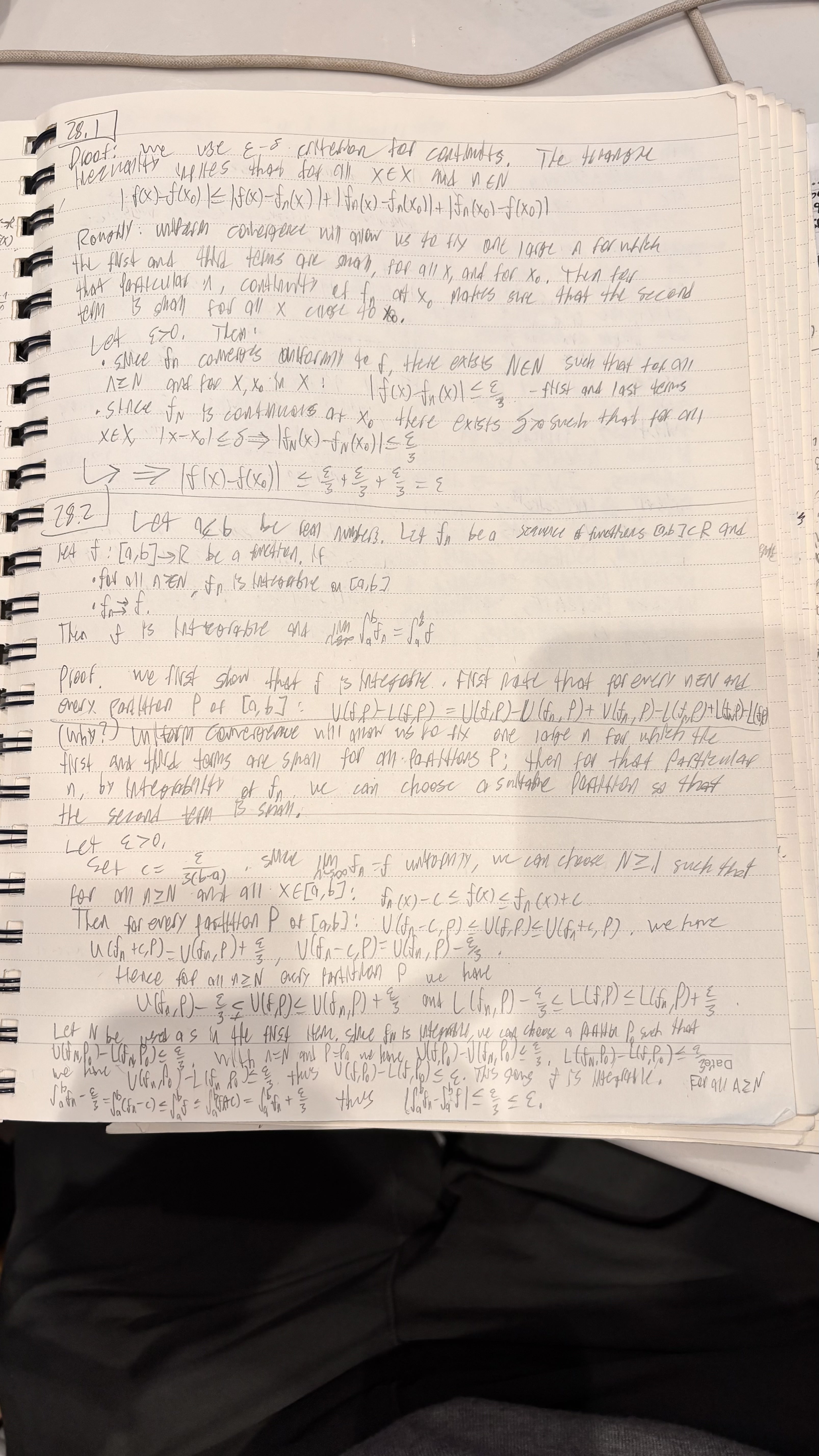
Definition 23.1 (Pointwise Convergence): A sequence of functions $(f_n)$ defined on a set $D$ converges pointwise to $f$ on $D$ if for every $x \in D$: $$\lim_{n \to \infty} f_n(x) = f(x)$$ Notation: $f_n \to f$ pointwise. Critique: Pointwise convergence is “weak.” It does not preserve properties like continuity. For example, $f_n(x) = x^n$ on $[0, 1]$ consists of continuous functions, but the limit is discontinuous (0 on $[0, 1)$, 1 at $x=1$).
Uniform Convergence
Uniform convergence requires the “speed” of convergence to be independent of $x$. The entire graph of $f_n$ must eventually fit inside an $\epsilon$-tube around $f$.
Definition 24.1 (Uniform Convergence): A sequence $(f_n)$ converges uniformly to $f$ on $D$ if for every $\epsilon > 0$, there exists an $N \in \mathbf{N}$ such that for all $n \geq N$ and for all $x \in D$: $$|f_n(x) - f(x)| < \epsilon$$ Notation: $f_n \rightrightarrows f$ uniformly. Key Difference: In pointwise, $N$ depends on both $\epsilon$ and $x$ ($N(\epsilon, x)$). In uniform, $N$ depends only on $\epsilon$ ($N(\epsilon)$).
Theorem 24.2 (Sup-Norm Criterion): Let $M_n = \sup { |f_n(x) - f(x)| : x \in D }$. Then $f_n \to f$ uniformly on $D$ if and only if $\lim_{n \to \infty} M_n = 0$.
- Usage: This is the standard calculation method. Find the maximum distance between $f_n$ and $f$, and check if that maximum goes to 0.
Theorem 24.3 (Cauchy Criterion for Uniform Convergence): $(f_n)$ converges uniformly on $D$ if and only if for every $\epsilon > 0$, there exists $N$ such that for all $n, m \geq N$ and all $x \in D$: $$|f_n(x) - f_m(x)| < \epsilon$$ .
4.2 Uniform Convergence and Continuity (Section 24)
This is the main reason we care about uniform convergence: it preserves continuity.
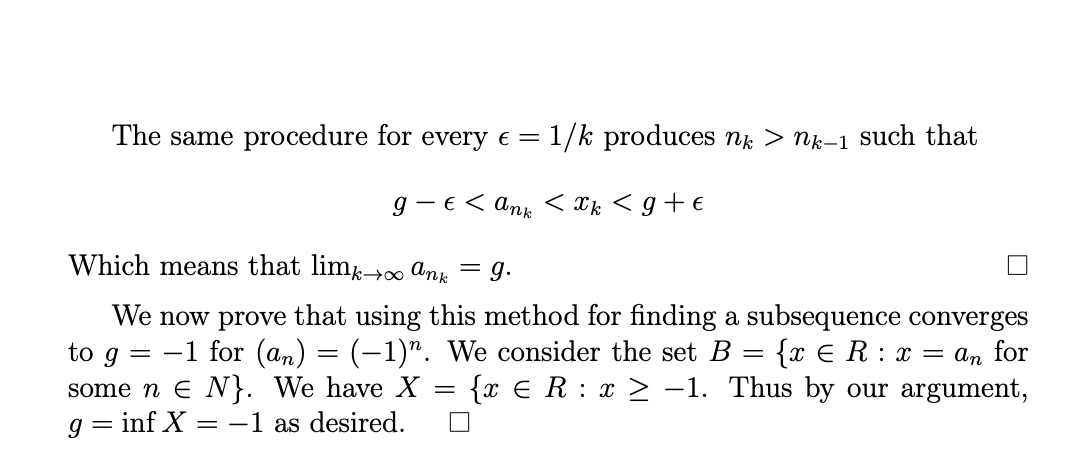
Theorem 24.4 (Continuous Limit Theorem): Let $(f_n)$ be a sequence of continuous functions on $D$. If $f_n$ converges uniformly to $f$ on $D$, then the limit function $f$ is continuous on $D$.
- Contrapositive: If $f_n$ are continuous but the limit $f$ is discontinuous, the convergence is not uniform. (Example: $x^n$ on $[0,1]$).
- Note: This theorem justifies “swapping limits”: $\lim_{x \to c} \lim_{n \to \infty} f_n(x) = \lim_{n \to \infty} \lim_{x \to c} f_n(x)$.
4.3 Uniform Convergence and Integration (Section 25)
Does $\int (\lim f_n) = \lim (\int f_n)$? Not always—unless we have uniform convergence.
Theorem 25.1 (Integration Theorem): Let $f_n$ be integrable functions on $[a, b]$. If $f_n$ converges uniformly to $f$ on $[a, b]$, then $f$ is integrable and: $$\lim_{n \to \infty} \int_a^b f_n(x) dx = \int_a^b f(x) dx$$
- Warning: Pointwise convergence is not enough. You can have sequences where the integral of the limit is 0, but the limit of the integrals is 1 (e.g., “moving bump” functions).
4.4 Uniform Convergence and Differentiation (Section 25)
Swapping derivatives is harder than swapping integrals. Uniform convergence of $f_n$ is not enough; we need uniform convergence of the derivatives $f’_n$.
Theorem 25.2 (Differentiation Theorem): Let $(f_n)$ be differentiable functions on $[a, b]$ such that:
- $(f_n(x_0))$ converges for some point $x_0$.
- The sequence of derivatives $(f’n)$ converges uniformly to a function $g$ on $[a, b]$. Then $(f_n)$ converges uniformly to a function $f$, $f$ is differentiable, and $f’(x) = g(x)$. $$\left( \lim{n \to \infty} f_n(x) \right)’ = \lim_{n \to \infty} f’_n(x)$$ .
4.5 Series of Functions (Section 26)
We apply the previous concepts to infinite series $\sum g_n(x)$.
Definition 26.1 (Convergence of Series): The series $\sum_{n=1}^{\infty} g_n(x)$ converges uniformly on $D$ if the sequence of partial sums $S_k(x) = \sum_{n=1}^k g_n(x)$ converges uniformly.
Theorem 26.2 (Term-by-Term Continuity/Integration): If continuous functions $g_n$ sum to $S(x)$ uniformly, then $S(x)$ is continuous and: $$\int_a^b \sum g_n(x) dx = \sum \int_a^b g_n(x) dx$$
The Weierstrass M-Test
This is the most critical tool for proving a series of functions converges uniformly. It reduces the problem to testing a series of numbers.
Theorem 26.3 (Weierstrass M-Test): Let $(g_n)$ be a sequence of functions on $D$. Suppose there exists a sequence of constants $M_n \geq 0$ such that:
- $|g_n(x)| \leq M_n$ for all $x \in D$.
- The series of numbers $\sum_{n=1}^{\infty} M_n$ converges. Then the series $\sum g_n(x)$ converges uniformly (and absolutely) on $D$.
- Example: $\sum \frac{\sin(nx)}{n^2}$ converges uniformly because $|\frac{\sin(nx)}{n^2}| \leq \frac{1}{n^2}$ and $\sum \frac{1}{n^2}$ converges ($p$-series with $p=2$).
4.6 Power Series (Section 26)
Power series are a special, well-behaved class of function series.
Theorem 26.4 (Radius of Convergence): For any power series $\sum a_n x^n$, there exists $R \in [0, \infty]$ such that:
- The series converges absolutely if $|x| < R$.
- The series diverges if $|x| > R$.
- $R = 1 / \limsup |a_n|^{1/n}$ (Hadamard Formula).
Theorem 26.5 (Uniform Convergence of Power Series): If a power series has radius of convergence $R > 0$, it converges uniformly on any closed interval $[-r, r]$ where $0 < r < R$.
- Consequence: Power series define continuous, differentiable, and integrable functions inside their radius of convergence. You can differentiate them term-by-term.